


Pairs trading is one of the most commonly used market neutral strategies. Over the last few years, several hedge funds have used different ways to successfully implement this trading strategy. The most extensively used techniques (correlation, distance, stochastic, stochastic differential residual and cointegration) use different methodologies and statistical tools to determine the two key elements of the strategy: pairs selection and the establishment of the long-term relationship between them. The purpose of this paper is to analyze the process of selecting pairs and determining the residual series using each one of the different techniques and comparing the outputs. Results indicate that far from being differentiated systems, relationships exist between the various techniques in terms of pairs selection and residual series creation. However, some techniques are more efficient at creating residual series than others, which then means that these techniques would have the highest probabilities of generating profits. The analysis concludes that cointegration is the most efficient method of structuring a pairs trading strategy.
Pairs trading, together with statistical arbitrage and risk arbitrage, has been one of the strategies most commonly used by hedge funds since the end of the 1990s (Nicholas, 2004). This type of strategy seeks to obtain profits from inefficiencies existing in the market, irrespective of whether it is a bull, bear or neutral market. Pairs trading consists of the simultaneous opening of long and short positions in two assets with a balance point between them. In this way, the earnings from a long position cover the losses from a short position and vice versa, meaning that the market risk is close to zero, as is the joint beta strategy. Therefore, the key elements that determine the success of a trade consists of determining the balance point between two securities and the point in time that prices move sufficiently away from the balance point to take positions. Pairs trading is not without risks as a miscalculation of these two elements can lead to a failure of the strategy (Opiela, 2004). Securities volatility is an additional risk that needs to be considered, even if there is a high degree of correlation between the securities (Whistler, 2004). Nevertheless, pairs trading can be used to not only generate profits regardless of market trend, but also to balance a portfolio given its market neutral properties. But to optimize trading results, it is necessary to first select the best method to implement a pairs trading strategy. There are five main techniques that can be utilized to execute a pairs trading strategy. These are: correlation, distance, stochastic, stochastic differential residual and co-integration although other authors mention others such as the machine learning and the time-series methods (Krauss, 2017).
These five techniques have been developed and proposed by different authors, however there have been no studies that analyze all of them jointly and under the same conditions. Accordingly, it is necessary to take a general and objective approach to be able to compare and contrast the properties of each one in relation to one another.
To do so, all techniques were compared, by performing an analysis of how pairs are chosen and how the balance point is determined as measured by the residual series. This allowed for the comparison of similarities that helped to determine the most efficient technique in each of the key aspects, given that until now, there have been no detailed comparative studies of the different techniques used to develop a pairs trading strategy. The sole exception is the study by Jurek and Yang (2007) which compared the results obtained from the distance and the stochastic techniques. This, then, is the first comprehensive study in which all five techniques are analyzed for interrelationships and to determine each one's strengths and weaknesses.
The remainder of the paper is organized as follows. The second section describes the theoretical aspects of pairs trading. The third section presents the data used and outlines the empirical techniques. The fourth section shows empirical results and the final section presents conclusions.
2TheoryThe principal challenge faced by financial investors using a pairs trading strategy is to find pairs of assets, be they stock, debentures, futures, currency, etc. with sound and lasting statistical relationships, based on the assumption that the different financial assets are, more or less, related (Arfaoui & Ben Rejeb, 2017). If the relationships are not stable in the medium or long-term, the investment system may incur substantial losses. The evolution of the main techniques includes theoretical components that relate different timeframes over which the relationships between a pair of assets break down. The most widely used include statistical tools, such as distance and correlation, stochastic and mathematical processes such as the stochastic and stochastic differential residual and statistical and econometric processes, such as that of co-integration (Do & Faff, 2010).
The correlation technique used by Wong (2010) chooses pairs of stocks according to the correlation coefficient existing between them and determines the residual series by means of a ratio of prices. This system has been used by different authors such as Ehrman (2006). With a given pair of stocks A and B, a ratio between their prices is used to generate the residual series:

The distance technique was developed and revised by Gatev, Goetzmann, and Rouwenhorst (2006). Their work is considered by many authors as the best-known work of pairs trading (Smith & Xu, 2017). It determines the pairs to be used by means of the distance between them, such distance being the total sum of squares of the difference between the standardized prices of both assets. The residual series is determined by the difference in standardized prices. Based on their work, Do and Faff (2010) developed a profitable pairs trading strategy.
The distance between each pair of assets is determined by:
where D is the distance between both assets, PAi is the standardized price of asset A at moment i and PBi is the standardized price of asset B at moment i.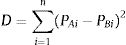
The standardized price of an asset is determined by:
where Pit is the standardized price of asset i at moment t, Pt is the price of the asset at moment t, E(Pi) is the mean or expected value of asset i and σi is the volatility or standard deviation of asset i.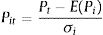
The residual series is determined by the standardized price difference between both assets:

The stochastic technique is based on the Hornstein–Uhlenbeck process and assumes a stationary residual series according to:
where k indicates the speed at which the residual series converges on its mean.
This was later used by Kanamura, Rachev, and Fabozzi (2008) and Jurek and Yang (2007) who, in addition, claimed to have achieved better results than those obtained by Gatev et al. (2006) based on a simulation of data. The residual series is established with the difference in price logarithms using the formula:
The stochastic differential residual technique developed by Do, Faff, and Hamza (2006) uses the CAPM and APT theoretical models to determine the balance between the assets. The residual series is obtained with:
where RtA is the profitability of asset A at moment t, RtB is the profitability of asset B at moment t, Γ is the difference between the betas of both assets and rm is the profitability of the reference market, measured by the index.
Finally, the co-integration technique used by Vidyamurthy (2004) establishes the relationship between assets based on the concept of co-integration developed by Engle and Granger (1987). The cointegration equation is determined by formula:

And the residual series can be written as the equation:
where α1 is the cointegration coefficient.3Data and methodology3.1Data and sample set used
Stocks within the US financial sector, specifically, the SP500 bank subgroup, were the sample set chosen for this study. This subgroup was chosen based on the recent economic crisis that severely punished the international banking industry, partly because of its high exposure to the mortgage and real estate markets. In addition, the banking sector is one of the most representative sectors of the economy, reaching almost 7% of worldwide GNP (World Bank, 2014). The total number of potential pairs analyzed in the study was determined by the formula:
where P is the number of possible resulting pairs and n is the number of stocks to be analyzed.
The sample period over which each technique was analyzed extended from January 1, 2008 to December 31, 2013. This time frame was chosen in order to more strongly contrast a market neutral investment strategy such as pairs trading, due to the major stock market fluctuations from the beginning of the economic crisis at the end of 2007 in which even the most advanced statistical tools of risk measure, as VaR, had shown to be inefficient and weak (Muela, Martin, & Sanz, 2017). Pairs trading is one of the most suitable strategies under current financial conditions that feature an unstable political environment and a high degree of uncertainty in the financial markets and the global economy (Ehrman, 2006).
3.2Methodology used by each technique for pairs selectionCorrelation: to determine the pair of stocks to be used, the correlation coefficient of all the pairs studied was calculated and the pair showing the highest degree of correlation was chosen.
Distance: to determine the pair of stocks to be used, the standardized prices of each pair of stocks and the distance between them were calculated according to formula (2) and (3). The pair of stocks chosen was the one that had the least distance between them.
Stochastic: to determine the pair of stocks to be used, the pair with the highest mean reversion was chosen; this being the pair with the highest k coefficient.
Stochastic differential residual: the pair of stocks to be used was the one with the lowest Γ coefficient, which measures the betas of both assets.
Cointegration: to determine the pair of stocks to be used, the pairs that were cointegrated were chosen. If there were several cointegrated pairs, the one whose residual function showed the highest degree of mean reversion was chosen, in other words, the one that showed the best result from the stationary test. A pre-selection of stocks based on the distance measurement system proposed by Vidyamurthy (2004) was not carried out, but rather all pairs were analyzed and those that passed the Johansen cointegration test were chosen (Johansen, 1989).
3.3Methodology used by each technique for price residual series formationCorrelation: the price residual series was formed by a quotient between the prices of both stocks according to formula (1). To simplify, the higher of the two prices was used as the numerator to obtain results above one at the beginning of the study.
Distance: the price residual series was formed by the difference between the standardized prices of both assets according to formula (4). For simplicity, we chose the highest figure first, to obtain positive results at the beginning of the study.
Stochastic: the residual series was created by the difference between the price logarithms of both stocks according to formula (6). For simplicity, we chose the highest figure first, to obtain positive results at the beginning of the study.
Stochastic differential residual: the residual series was calculated according to formula (7) with the first figure of the equation being the one that showed the highest profitability in order to obtain positive results at the beginning of the study.
Cointegration: the residual series was obtained using the equation from a linear regression according to formula (9). In this case, the first figure used corresponded to the endogenous variable of the model, followed by the long-term balance value and, finally, the exogenous variable of the model.
4ResultsThe following are the results obtained, according to the different analyses carried out. We extracted different types of results: firstly, with respect to the selection process of the pair of stocks and secondly, to the creation of the residual series of a given pair of stocks.
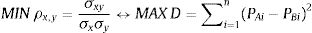
Regarding the technique used for pairs selection, we found that the correlation and the distance methods systematically choose the same pair of stocks and in the same order. In other words, the pair of stocks with the highest correlation is also the one with the least distance between them. Provided the pair of stocks x and y are equivalent to the A and B stocks, the latter pair standardized. This means that if we analyze the same pair of stocks and this pair has the highest correlation coefficient (ρx,y) of all the potential pairs, it will also have the least distance (D) of all potential pairs. We can therefore state that the value of the correlation coefficient and the distance between two pairs of stocks is inversely related:
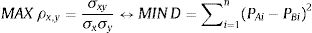
This relationship is maintained until the pair of stocks with the lowest correlation coefficient (ρx,y) is reached which, in turn, has the highest value in distance (D). We can also therefore establish that:
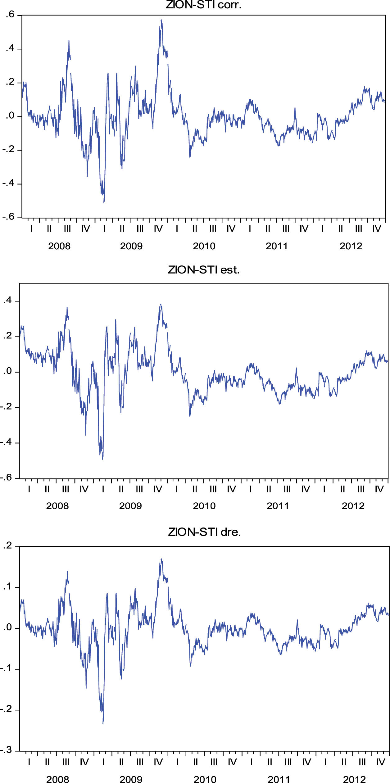
With regard to the creation of the residual series, from the study carried out we can infer that the correlation, stochastic and stochastic differential residual techniques generate the same residual series with a different scale. This equivalence in how the residual series is constructed and the difference in scale can be seen clearly in Fig. 1. In this case, as an example, the residual series generated by the pair of Sun Trust Banks (STI) and Zion's Bankscorp (ZION) is used during the analysis period. In the following series, the mean is adjusted to zero, in order to eliminate the independent term effect.
 and Sun Trust Banks (STI) (*).")
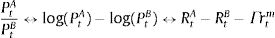
Nevertheless, this change in scale does not affect the entrance and exit signals, as the results obtained by applying each of the three-residual series is exactly the same for a given pair of stocks. This residual series equality obtained is clearly observed between the correlation and stochastic techniques, given the way it is constructed: correlation establishes a ratio according to formula (1) while stochastic establishes the difference in price logarithms using formula (5), which can be re-written as:

Therefore, the residual series created using the correlation and stochastic methods are the same, with a change of logarithmic scale. With respect to the stochastic differential residual method, the residual series is obtained according to formula (7).
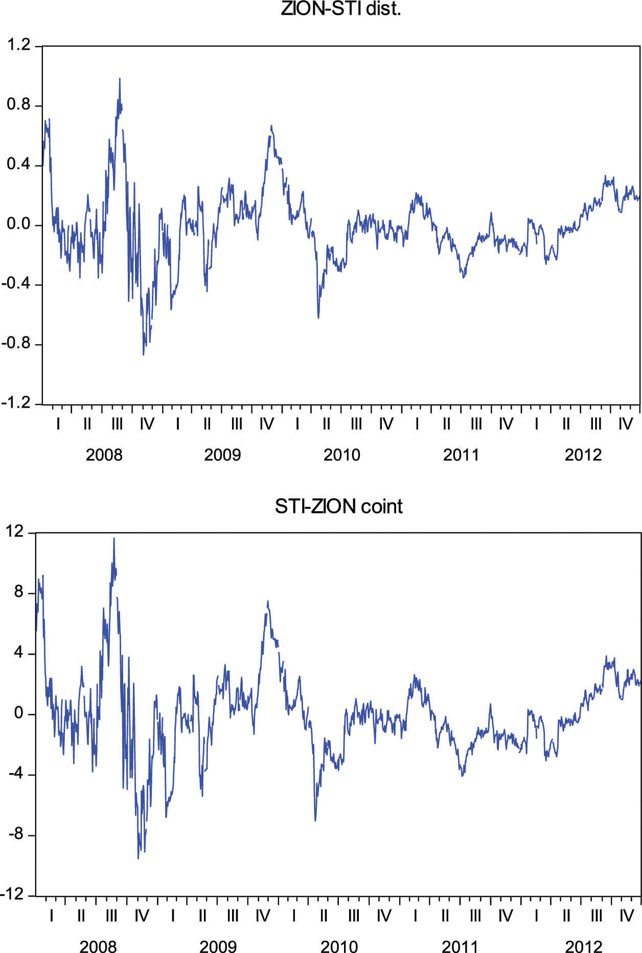
The distance and cointegration techniques generate the same residual series with a different scale for a given pair of stocks. The residual series using the distance technique is determined by the standardized price difference between both assets according to formula (4) while in the cointegration technique the residual series can be written as Eq. (9). This equivalence in how the residual series is obtained and the difference in scale can be seen clearly in Fig. 2, with the given pair of Sun Trust Banks (STI) and Zion's Bankscorp (ZION) during the period of analysis.
 and Zion's Bankscorp (ZION) (*).")
We can therefore state that the correlation, stochastic and differential residual stochastic residual series are equivalent and that:
We can also state that the residual series created using the distance and cointegration techniques are equivalent:

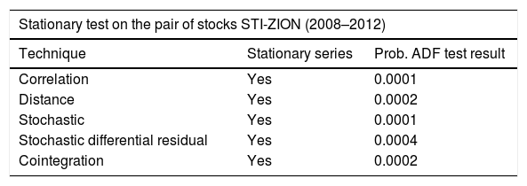
Finally, it must be pointed out that the residual series generated by distance and cointegration is a series similar to those created by correlation, stochastic and stochastic differential residual; with a correction of the series trend, meaning that the results of the stationary tests in series with a trend are, in general, better than those obtained with the other three techniques. The residual series formed by Zion's Bankscorp. (ZION) and Sun Trust Banks (STI) does not show a clear trend, as observed directly from Figs. 1 and 2, therefore in this case the stationary tests on all the residual series show similar results, as seen in Table 1.
Results of the ADF stationary test and probability of the STI-ZION residual series.
| Stationary test on the pair of stocks STI-ZION (2008–2012) | ||
|---|---|---|
| Technique | Stationary series | Prob. ADF test result |
| Correlation | Yes | 0.0001 |
| Distance | Yes | 0.0002 |
| Stochastic | Yes | 0.0001 |
| Stochastic differential residual | Yes | 0.0004 |
| Cointegration | Yes | 0.0002 |
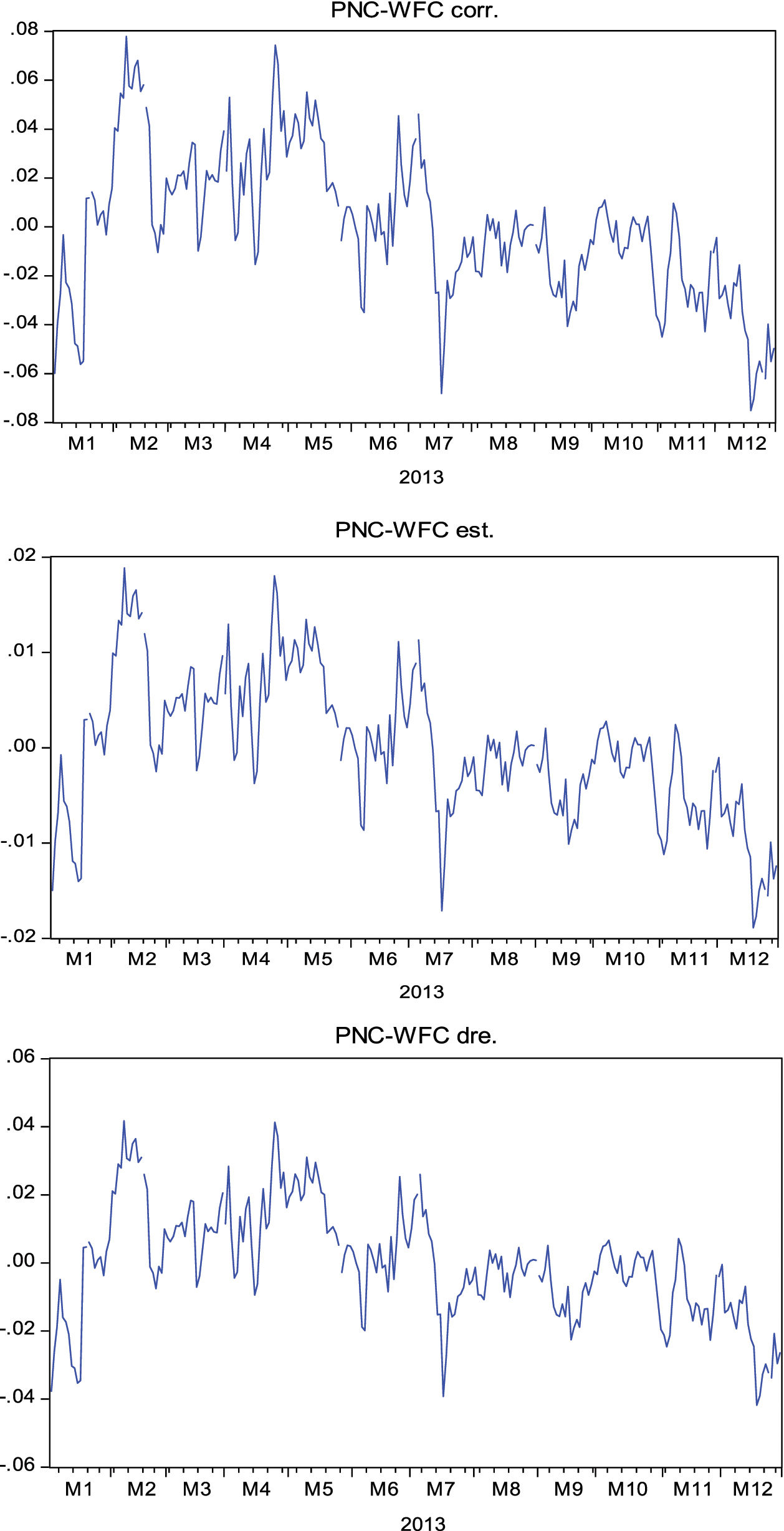
In order to confirm the results, the residual series formed by the pair of PNC Financial Services (PNC) and Wells Fargo (WFC) was analyzed during the test period. An analysis of the graph shows that the residual series has a slightly decreasing trend. This equivalence in how the residual series is obtained from the correlation, stochastic and stochastic differential residual techniques and the difference in scale can be seen clearly in Fig. 3, with a given pair of PNC Financial Services (PNC) and Wells Fargo (WFC) during the 2013 time frame. In these residual series, the mean was zero, to eliminate the independent term effect.
 and Wells Fargo (WFC) (*).")
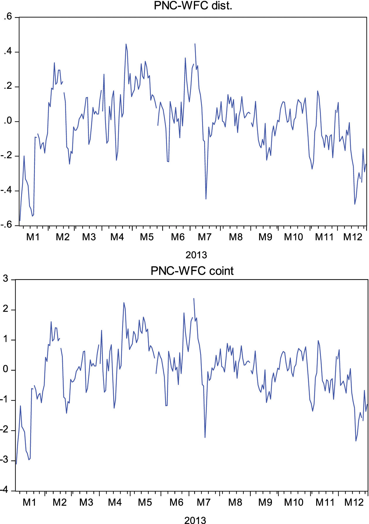
Similarly, the way in which the residual series was obtained using the distance and cointegration techniques and the difference in scale can be clearly seen in Fig. 4, given the pair of PNC Financial Services (PNC) and Wells Fargo (WFC) during the 2013 period.
 and Wells Fargo (WFC).")
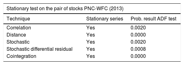
In this case, the decreasing trend of the residual series is observed as more gradual in contrast to those formed by the three previous techniques. It is in this type of series with a trend that it can be directly observed that the results provided by distance and cointegration are better. In the case of a trend in the residual series, the lowest values from the test are also always those obtained from the residual series using the distance and cointegration techniques, as shown in Table 2.
Results of the ADF stationary test and probability of the PNC-WFC residual series.
| Stationary test on the pair of stocks PNC-WFC (2013) | ||
|---|---|---|
| Technique | Stationary series | Prob. result ADF test |
| Correlation | Yes | 0.0020 |
| Distance | Yes | 0.0000 |
| Stochastic | Yes | 0.0020 |
| Stochastic differential residual | Yes | 0.0008 |
| Cointegration | Yes | 0.0000 |
The results obtained show that a pairs trading strategy based on the distance and cointegration techniques generates residual series with better properties than the other techniques for a given pair of stocks. With regard to the method of choosing pairs of stocks, cointegration requires a comprehensive analysis of each potential pair, to choose the pair with the highest degree of cointegration and, therefore results in a residual series with better properties. Accordingly, it can be said that cointegration chooses stocks in a more accurate and complete way than distance and is therefore preferred.
It was also found that the stochastic technique used by Elliott, Van Der Hoek, and Malcolm (2005), Jurek and Yang (2007) and Kanamura et al. (2008) is based on the assumption that the residual series used by the strategy is represented by an Ornstein-Uhlenbeck stochastic model, in which the k, θ and σ parameters are constant, which is extremely difficult in practice. In fact, the greatest challenge faced by pairs trading consists in choosing stocks that can form a series with these properties.
Furthermore, it was proven that pairs trading, using any of the techniques analyzed, was market neutral and that suitable residual series were found in both the time frames analyzed. This feature clearly distinguishes it from other traditional investment strategies, thus making it an interesting investment strategy in terms of risk diversification and as an additional tool in the process of investment portfolio asset allocation. Pairs trading can also be used by portfolio managers with different levels of leverage in order to adjust the risk of the strategy. It should be noted that the analysis of the stocks was performed manually, with the implications that this portends. This limitation can be avoided by programming the strategy to incorporate different timeframes, especially for intraday trading, given the speed that this type of trading requires. The timeframe used for the analysis was selected because of the high volatility of the market during the years of the economic crisis. It would be interesting to test a pairs trading strategy during a timeframe with less volatility and to compare the results.
