Cost efficiency analysis of Swedish financial enterprises: An empirical investigation

Abstract

In this paper, our research question that could analyze how efficiency in Swedish financial enterprises has changed since the banking crisis in 1993. We estimate the time-invariant and time-variant efficiencies of Swedish financial enterprises with four different estimators. These estimators are the Pooled Model (Aigner et al., 1977), the fixed effects model (Schmidt & Sickles, 1984), the random effects model (Battese & Coelli, 1995) and the TRUE fixed effects model (Greene, 2005) efficiency estimators. We predict cost function by employing panel stochastic frontier approach. These allow us to construct cost efficiency.

1

Introduction

Before 1980, financial markets were highly regulated in Sweden. Much credit flowed outside the regulated market and challenged the traditional role of banks. In response, banks tried to bypass interest rate regulations by establishing their own finance companies, which formed an important part of the gray credit market (Berg et al., 1993). The term ‘gray economy’, however, refers to workers being reimbursed under-the-table, without paying income taxes or contributing to such public services as Social Security and Medicare. It is sometimes referred to as the underground economy or “hidden economy” in Sweden (Biljer, 1991).

As the regulations were increasingly considered to be largely ineffective, the authorities initiated a financial liberalization process in the late 1970s that proceeded through the 1980s. Credit and bond markets were deregulated first; regulations on international transactions were removed next. The system of liquidity ratios for banks was abandoned in 1983 and the ceilings on commercial bank lending were removed in 1985. At the same time, restrictions on lending rates were lifted. By 1989, all remaining foreign exchange restrictions had been removed (Dress & Pazarbasioglu, 1998).

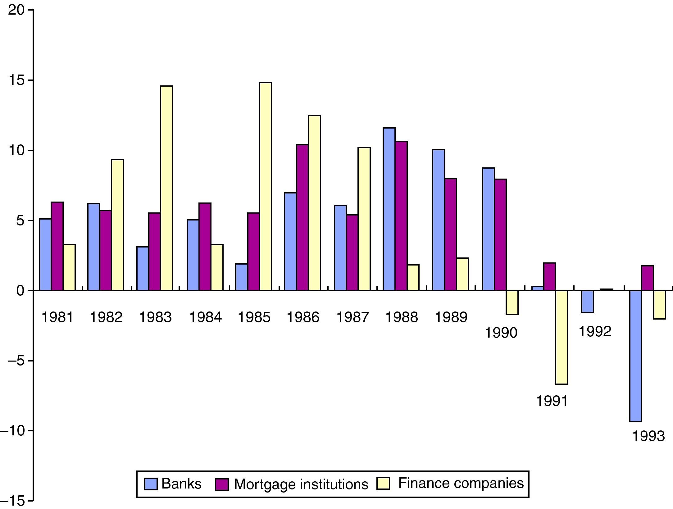
The immediate impact on consumption and investment appears to have been limited. Expressed differently, the rationing effects of the abolished regulations do not seem to have been quantitatively important to the real decisions of households and corporations. On the other hand, financial flows were undoubtedly affected in an important way (Ahmet et al., 2011). Credits were increasingly channelled by financial institutions, such as banks and mortgage institutions, rather than directly between firms (for example trade credits) and households (for example seller financed housing loans). Loans were also increasingly used for high-leverage financial investments. These effects on financial flows may, if their impact on asset prices is any indication, have affected the banking crisis (Fig. 1) (Englund, 1999).

Fig. 1.

Lending from banks, mortgage institutions and financial companies (percentage changes).

We estimate the time-invariant and time-variant efficiencies of Swedish financial enterprises. These estimators are the Pooled Model (Aigner, Lovell, & Schmidt, 1977), the fixed effects model (Schmidt & Sickles, 1984), the random effects model (Battese & Coelli, 1995) and the TRUE fixed effects model (Greene, 2005). We predict cost function by employing the panel stochastic frontier approach. This allows us to build cost efficiency.

In this research, the cost measure was estimated for the panel data utilising six different financial enterprises from 1996 to 2011. These financial enterprises comprise banks (including commercial banks, branches of foreign banks in Sweden and saving banks), credit market companies, housing credit institutions, other mortgage institutions, other credit market companies and securities brokerage companies. In the next section, we conduct a literature review of the stochastic frontier approach and related banking. Section 3 describes the stochastic frontier methodology. Section 4 provides data and empirical results of the Swedish banking case. Finally, Section 5 makes conclusions.

2

Literature review

The stochastic frontier approach (SFA) pertains to the theoretical literature on productive efficiency that began in the 1950s with the work of Koopmans (1951), Debreu (1951) and Shephard (1953). Koopmans provides a definition of technical efficiency: a producer is technically efficient if and only if it is impossible to produce more of any output without producing less of some other output or without using more of some input. Debreu and Shephard introduce distance functions as a way of modelling multiple-output technology and – more importantly, from our perspective – as a way of measuring the radial distance of a producer from a frontier in either an output-expanding direction (Debreu) or an input-conserving direction (Shephard). The association of distance functions with technical efficiency measures is pivotal in developing the efficiency measurement literature.

Farrell (1957) was the first to measure productive efficiency empirically (drawing inspiration from Koopmans and Debreu but clearly not from Shephard). He also provides an empirical application for U.S. agriculture, although he did not use econometric methods.

Aigner et al. (1977) (ALS hereafter) propose a model in which errors were allowed to be both positive and negative but in which positive and negative errors could be assigned different weights. Ordinary least squares emerge as a special case of equal weights, and a deterministic frontier model emerges as another special case. They consider estimation for the case in which the weights are known and for the more difficult case in which the weights are unknown and are to be estimated with the other parameters in the model. They do not estimate the model and, to our knowledge, no one else has done so either. Nonetheless, there is a short step from the Aigner, Amemiya and Poirier model (with larger weights attached to negative errors) to a comprised error stochastic production frontier model. The step took a year. SFA originated with two papers published nearly simultaneously by two teams on two continents. The ALS paper is in fact a merged version of a pair of remarkably similar papers: one by Aigner and the other by Lovell and Schmidt. The ALS and Meeusen and van den Broeck (MB hereafter) papers are themselves very similar. Both papers were three years in the making and both appeared shortly before a third SFA paper by Battese and Corra (1977), the senior author of which had been a referee of the ALS paper. These three original SFA models share the comprised error structure mentioned previously, and each was developed in a production frontier context.

Schmidt and Sickles (1984) apply fixed effects and random effects models to estimate the efficiencies of the firms. In their study, the efficiencies of the firms are assumed to be time-invariant, which might not be a proper assumption for long panel data. Accordingly, they consider estimating a stochastic frontier production model, given panel data. They provide various estimators that depend on whether one is willing to assume that technical inefficiency (the individual effect, in panel-data jargon) is uncorrelated with the regressions and whether one is willing to make specific distributional assumptions for the errors. They show how to test these assumptions.

Battese and Coelli (1995) propose a model for technical inefficiency effects in a stochastic frontier production function for panel data. Provided the inefficiency effects are stochastic, the model allows for the estimation of both technical change in the stochastic frontier and time-varying technical inefficiencies.

Greene (2005) proposes extensions that circumvent two shortcomings of fixed and random effects estimator approaches. The conventional panel data estimators assume that technical or cost inefficiency is time invariant. Second, the fixed and random effects estimators force any time invariant cross unit heterogeneity into the same term that is being used to capture the inefficiency. Inefficiency measures in these models may pick up heterogeneity in addition to or even instead of inefficiency.

Berger and Mester (1997) survey 130 studies that apply frontier efficiency analysis to financial institutions in 21 countries. They do this to summarise and critically review empirical estimates of financial institution efficiency and to try to arrive at a consensus view. They find the various efficiency methods do not necessarily yield consistent results and suggest some ways that these methods might be improved upon to yield findings that are more consistent, accurate and useful. Almost all of the studies that estimate efficiency and then regress it on sets of explanatory variables have been unable to explain more than just a small portion of the total variation. While some differences have been found, little published information exists about those influences that are under direct management control, such as the choice of funding sources wholesale versus retail orientation, etc. Cost and productive efficiency average 84 percent when parametric estimation techniques are used and 72 percent when nonparametric techniques are used.

In the Swedish case, Battese et al.’s (2000) paper aims to analyse the impact of the deregulation of Swedish banking industry in the mid-1980s and the consequent banking crisis on productive efficiency and productivity growth in the industry. An unbalanced panel of Swedish banks is studied over the period of 1984–1995. A total of 1275 observations are analysed for 156 banks observed. The inefficiency effects in the labour-use frontier are modelled in terms of the number of branches, total inventories and the type of bank and year of observation. The technical inefficiencies of the labour use of Swedish banks are significant, with mean inefficiencies a year estimated to be between about 8 and 15 percent over the years of study.

Gjirja (2004) analyses the impact of deregulation and the subsequent banking crisis on the efficiency of labour in the Swedish banking sector. A translog stochastic frontier model is adopted in order to estimate the labour input requirement function and to assess bank technical efficiency. Furthermore, the parameters of the stochastic frontier function are simultaneously estimated with the parameters of a model for the technical inefficiency effects. The analysis suggests that there is capacity for substantial labour efficiency improvements in the Swedish banking industry. It is also shown that deregulation positively affects productivity growth. However, no such positive impact is found on labour use efficiency. In addition, the banking crisis affected the efficiency of labour utilization in Swedish banks in a negative way, considering the involved outputs and inputs (“effects of deregulation and banking crisis on the labour use efficiency in Swedish banking industry”). The fast pace of changes in the economic environment and the increasing globalization of financial services dictate an increase in the awareness of financial institutions regarding their economic performance.

Papadopoulos (2010) explores the issue of efficiency in Scandinavian banking by applying the Fourier functional form and the stochastic cost frontier approach to calculate inefficiencies for Finnish, Swedish, Danish and Norwegian banks from 1997 to 2003. The findings suggest that the largest banks are the least efficient, and the smallest banks are the most efficient. The strongest economies of scale are displayed by Danish banks, while the weakest economies of scale are reported by Finnish banks. The findings suggest that medium-sized banks report the strongest economies of scale and the largest and smallest banks weaker economies of scale and therefore the notion that economies of scale increase with bank size cannot be confirmed. The impact of technical change in lessening bank costs (generally about 3% and 5, 4% an annual) systematically increases with bank size. The largest banks reap the greatest benefits from technical changes. Overall, the results show that the largest banks in their sample enjoy greater benefits from technical progress, although they do not have scale economy and efficiency advantages over smaller banks.

3

Methodology

One can obtain the cost efficiency of a bank by employing either nonparametric or parametric approaches. Nonparametric (non-stochastic) cost efficiency is calculated by employing linear mathematical programming techniques. On the other hand, parametric (stochastic) cost efficiency is derived from a cost function in which variable costs depend on input prices, quantities of variable outputs, random error and inefficiency.

where C_b stands for the financial enterprises’ total operational costs, y_i represents the vector of quantities of the financial enterprises’ variable outputs, p_k is the vector of prices of the financial enterprises’ variable inputs and εb is a composite error term, through which the cost function varies stochastically. The cost function provides an indirect representation of the possible technology because it is mainly a specification for the minimum cost of producing the output vector, y, given the cost drivers (such as price vector), p, in the input market, managerial inefficiency, some exogenous economics factors or pure luck (Kumbhakar & Lovell, 2003).

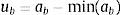
The term εb can be partitioned into two parts as follows:

where e_b refers to endogenous factors and u_b refers to exogenous factors that impact the cost of the bank production. Thus, the term u_b denotes a rise in the cost of bank production because of the inefficiency factor, which may result from the mistakes of management (i.e. non-optimal employment of the quantity or mix of inputs given their prices). On the other hand, e_b represents a temporary rise or fall in the bank's costs because of the random factor that a system from a data or measurement error or unexpected or uncontrollable factors (such as weather luck, labour strikes and war) that cannot be changed by the management (Lovell et al., 1982).

Firstly, Aigner et al. (1977) defines a firm's cost function as follows:

where f is a functional form and εb=ub+eb is the composite error term. Parametric and non-parametric efficiency techniques differ in terms of how to disentangle the comprised error term, εb. Non-parametric techniques assume that there is no error and attribute any deviation from the best practice bank's cost to inefficiency. On the other hand, parametric techniques assume that the inefficiencies follow an asymmetric distribution. That is, they assume that the half-normal and random errors follow a symmetric distribution, the standard normal. In other words, random factors are assumed to be identically distributed as normal variants, and the value of the error term in the cost function is equal to zero on the average. Thus, inefficiency scores are derived from a normal distribution N(0,σu2) but are truncated below zero. The underlying reason for the truncated normal distribution assumption is that inefficiencies cannot be negatively signed (Isik & Hassan, 2002).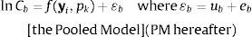

Secondly, in accordance with Schmidt and Sickles’ (1984) approach, the fit should be an ordinary (within-groups) OLS; this should be followed by a translation of the constants:

In Eq. (1.5), the definition of a_b amounts to counting the real efficiency firm in the sample. The definition of min(a_b) amounts to counting the most efficient firm in the sample as average efficient scores.

Thirdly, the Battese and Coelli (1988, 1992, 1995) model specification may be expressed as:

the e_b are random variables, which are assumed to be iid. N(0,σu2). They are independent of the u_b which are non-negative random variables that are assumed to account for technical inefficiency in cost function and to be independently distributed as truncations at zero of the N(μit,σu2) distribution:

where z_bt may influence the efficiency of a firm, and δ is parameters to be estimated.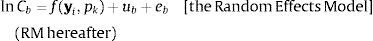

Battese and Coelli (1995) once again use the parameterisation from Battese and Corra (1977), replacing σe2 and σu2 with σ2=σe2+σu2 and.

The log-likelihood function of this model is presented in the appendix in the Battese and Coelli (1995).

This model specification also encompasses a number of other model specifications as special cases. If we set T =1, and z_bt contains the value one and no other variables (i.e. only the constant term), then the model reduces to the truncated normal specification, where δ0 (the only element in) will have the same interpretation as the μ parameter in Stevenson (1980). It should be noted, however, that the model is defined by Eqs. (1.6) and (1.7).

Finally, Greene (2003, 2004, 2005) reformulates the stochastic frontier specifically to explore these aspects, calling it the stochastic frontier model in a ‘true’ fixed effects formulation. The estimated parameters ρi,bj,cm are given the true values for the structural parameters in the model. A set of ‘true’ values for u_bt is generated for each firm and reused in every replication. These ‘inefficiencies’ are maintained as part of the data for each firm for the replications. The firm-specific values are produced using ubt•=|Ubt•| where Ubt• is a random draw from the normal distribution with a mean of zero and a standard deviation.¹ Thus, for each firm, the fixed data constant term a_i, the inefficiencies ubt• and the financial enterprises total operational costs data lnCbt* are produced using

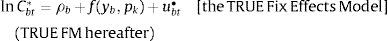
By this device, the underlying data to which we will fit the fixed effects model are actually generated by an underlying mechanism that exactly satisfies the assumptions of the TRUE fixed effects stochastic frontier model. Additionally, the model is based on a realistic configuration of the right-hand side variables. Each replication, r, is then produced by generating a set of disturbances ebtCbt*=ρb+f(yb,pk)+ubt* from the normal distribution, with mean 0 and standard deviation. The data that enter each replication of the simulation are then lnCbt(r)=lnCbt*+ebt*(r). The estimation was replicated 100 times to produce the sampling distributions. We computed the sampling error in the computation of the inefficiency for each of the 96 observations in each replication, dubt(r)=estimation ubt(r)−ubt*. The values are not scaled, as these are already measured as percentages (changes in log cost); we analyse the raw deviations, dubt(r). The mean of these 96 deviations is computed for each of the 100 replications (Greene, 2005).

We first need to specify a relationship (function) between bank production and bank cost in order to estimate the inefficiency u_b and random e_b factors of the composite εb error term. To that end, we specify banks as multi-product and multi-input firms and estimate the following translog cost function:

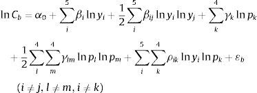
To that end, we specify banks as multi-product and multi-input firms and estimate the following translog cost function:

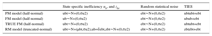
where ln is natural logarithm, C_b is the bth bank's total (interest and non interest) costs; y_i is the ith output; p_k is kth input price and εb is the composite error term.

The Technical Inefficiency Score (TIES hereafter) is measured in Table 1.

Table 1.

Econometric specifications of the stochastic cost frontier.

	State specific inefficiency ub, and zbt	Random statistical noise	TIES
PM model (half-normal)	ubt∼N+(0,σu2)	ebt∼N+(0,σe2)	ubtubt+ebt
FM model (half-normal)	ub∼N+(0,σu2)	ebt∼N+(0,σe2)	ubub+ebt
TRUE FM (half-normal)	ubt∼N+(0,σu2)	ebt∼N+(0,σe2)	ubtubt+ebt
RM model (truncated-normal)	ubt∼N+(μbt,σu2),ub=δzbt,zbt∼N+(0,σz2)	ebt∼N+(0,σe2)	zbtzbt+ebt

4

Data and definition of variables

4.1

Data and description of variables

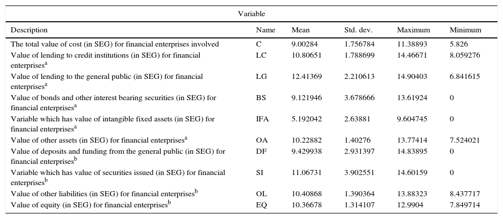
In this context, this core chapter uses the distribution free approach to estimate the levels of cost efficiency of individual financial enterprises in Sweden. We use the annual panel data of all the financial enterprises of Sweden from 1996 to 2011. These financial enterprises comprise banks (including commercial banks, branches of foreign banks in Sweden and saving banks), credit market companies, housing credit institutions, other mortgage institutions, other credit market companies and securities brokerage companies. The database of each enterprise has been aggregated by the Statistics Sweden. We use two distinct dependent and nine independent variables consisting of five outputs and four inputs. The maximum-likelihood estimates of the parameters of the model are obtained using a modification of the econometric software. Descriptive statistics of the key variables are presented in Table 2.

Table 2.

Descriptive statistics.

Variable
Description	Name	Mean	Std. dev.	Maximum	Minimum
The total value of cost (in SEG) for financial enterprises involved	C	9.00284	1.756784	11.38893	5.826
Value of lending to credit institutions (in SEG) for financial enterprises^a	LC	10.80651	1.788699	14.46671	8.059276
Value of lending to the general public (in SEG) for financial enterprises^a	LG	12.41369	2.210613	14.90403	6.841615
Value of bonds and other interest bearing securities (in SEG) for financial enterprises^a	BS	9.121946	3.678666	13.61924	0
Variable which has value of intangible fixed assets (in SEG) for financial enterprises^a	IFA	5.192042	2.63881	9.604745	0
Value of other assets (in SEG) for financial enterprises^a	OA	10.22882	1.40276	13.77414	7.524021
Value of deposits and funding from the general public (in SEG) for financial enterprises^b	DF	9.429938	2.931397	14.83895	0
Variable which has value of securities issued (in SEG) for financial enterprises^b	SI	11.06731	3.902551	14.60159	0
Value of other liabilities (in SEG) for financial enterprises^b	OL	10.40868	1.390364	13.88323	8.437717
Value of equity (in SEG) for financial enterprises^b	EQ	10.36678	1.314107	12.9904	7.849714

a

Output.

b

Input.

4.2

Empirical results

In this section, we present and discus the efficiency results obtained indirectly from a functional form regarding the costs of the financial enterprises.

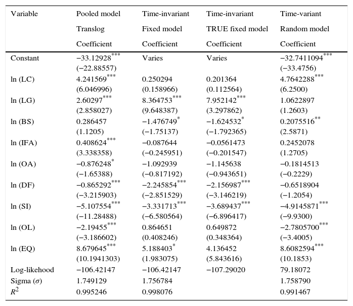
The estimation results of the frontier cost inefficient models that use the PM, the FM and the RM are given in Table 3.² Given that most of the variables are in logarithmic form, the coefficients can be interpreted as estimated elasticises. The results suggest that the lending to general public is quantity – elastic estimated elasticises of 2.60, 8.40, 7.95 and 1.05 for the PM, the FM, the TRUE FM and the RM. The results also suggest that the security issue is price (elastic), with an estimated elasticity of −5.10 for the PM, −3.33 for the FM, −3.68 for the TRUE FM and −4.91 for the RM.

Table 3.

Estimated coefficients of cost function (t-values in parentheses).

Variable	Pooled model	Time-invariant	Time-invariant	Time-variant
	Translog	Fixed model	TRUE fixed model	Random model
	Coefficient	Coefficient	Coefficient	Coefficient
Constant	−33.12928^*** (−22.88557)	Varies	Varies	−32.7411094^*** (−33.4756)
ln (LC)	4.241569^*** (6.046996)	0.250294 (0.158966)	0.201364 (0.112564)	4.7642288^*** (6.2500)
ln (LG)	2.60297^*** (2.858027)	8.364753^*** (9.648387)	7.952142^*** (3.297862)	1.0622897 (1.2603)
ln (BS)	0.286457 (1.1205)	−1.476749^* (−1.75137)	−1.624532^* (−1.792365)	0.2075516^** (2.5871)
ln (IFA)	0.408624^*** (3.338358)	−0.087644 (−0.245951)	−0.0561473 (−0.201547)	0.2452078 (1.2705)
ln (OA)	−0.876248^* (−1.65388)	−1.092939 (−0.817192)	−1.145638 (−0.943651)	−0.1814513 (−0.2229)
ln (DF)	−0.865292^*** (−3.215903)	−2.245854^*** (−2.851529)	−2.156987^*** (−3.146219)	−0.6518904 (−1.2054)
ln (SI)	−5.107554^*** (−11.28488)	−3.331713^*** (−6.580564)	−3.689437^*** (−6.896417)	−4.9145871^*** (−9.9300)
ln (OL)	−2.19455^*** (−3.186602)	0.864651 (0.408246)	0.649872 (0.348364)	−2.7805700^*** (−3.4005)
ln (EQ)	8.679645^*** (10.1941303)	5.188403^* (1.983075)	4.136452 (5.843616)	8.6082594^*** (10.1853)
Log-likehood	−106.42147	−106.42147	−107.29020	79.18072
Sigma (σ)	1.749129	1.756784		1.758790
R^2	0.995246	0.998076		0.991467

*

Coefficient is significantly different from zero at the 90% confidence levels (by Statistical Sweden).

**

Coefficient is significantly different from zero at the 95% confidence levels (by Statistical Sweden).

***

Coefficient is significantly different from zero at the 99% confidence levels (by Statistical Sweden).

In the cost translog function, the homogeneity condition is, the signs of the coefficients of the stochastic frontier are as expected, with the exception of the negative estimate of input variables (without the value of equity for three models) and the positive estimate of output variables. Results of the sum of all coefficients are negative for the cost function. In this connection, each model is provided the homogeneity condition in our estimations.

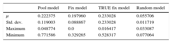
Table 4 provides descriptive statistics for the overall Swedish estimated ‘cost inefficiency scores’ for the 6 different financial enterprises from 1996 to 2011. This shows that the estimated u_b is about 12–38%. Then, the technical efficiency³ of financial enterprises is 94%, 77%, 81% and 78% for the RM, the TRUE FM, the FM and the PM.

Table 4.

Cost inefficiency scores.

	Pool model	Fix model	TRUE fix model	Random model
μ	0.222375	0.197960	0.233028	0.055706
Std. dev.	0.119003	0.088867	0.233028	0.011719
Maximum	0.048774	0.0	0.016417	0.033087
Minimum	0.771586	0.329265	0.528317	0.077064

Table 5 provides correlation among efficiency estimates of our models. Among the notable features of the results is the high correlation between the random model and the fixed model estimates. The pool model is lower in correlation across the two modelling platforms, time-varying and time-invariant effects. Then, the TRUE FM model has a very high correlation between the pool, the random and the fix models.

Table 5.

Correlation among inefficiency estimates.

	Pool model	Fixed model	TRUE fix model	Random model
Pool model	1
Fixed model	0.41568	1
TRUE fixed model	0.81814	0.71587	1
Random model	0.41923	0.98467	0.72694	1

We want to find the fit model in these estimators. We use hypothesis tests for our estimators. These tests show that the TRUE FM model is the fit model in our database. The Hausman test results support this finding. The following explanations are based on the TRUE fix model.

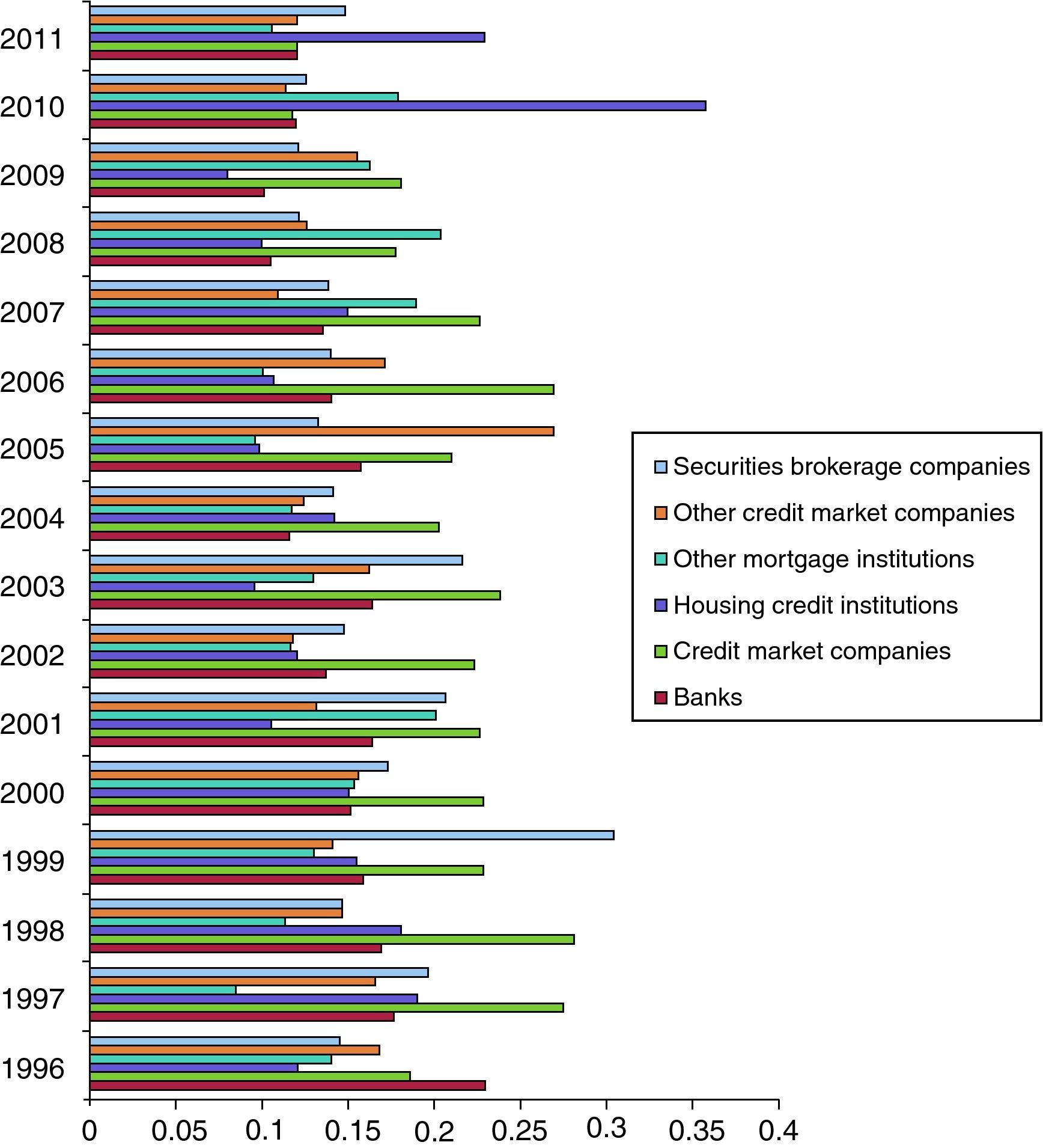
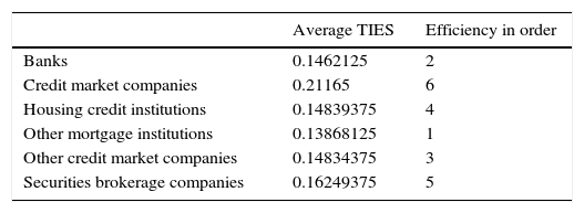
Fig. 2 provides a summary of the individual inefficiency scores of financial enterprises. Other credit market companies are less inefficient than other financial enterprises. This results show that other mortgage institutions are more successful in terms of cost-management than others. Next, Banks (saving, commercial and investment) are successful in these financial enterprises. Accordingly, the credit market companies have the worst efficiency scores in the financial system. Housing credit intuitions and credit market institutions are higher in inefficiency than the other four financial enterprises (Table 6). Housing credit intuitions and credit market institutions have especially been affected by some enterprise scandals. This affects efficiency for the housing credit intuitions. In 2011 and 2010, the inefficiency score of the housing credit intuitions was the highest of all the years. This means that the inefficiency score of the credit market institutions changed in 2010 and 2011. During these years (2010 and 2011), the inefficiency score of the credit market institutions were the lowest of all of the years. These events depend on the subprime mortgage crises of 2008 (Fig. 2).

Fig. 2.

Estimated ‘Individual Inefficiency of Financial Enterprises’ (the TRUE FM, from 1996 to 2011).

Table 6.

Average Technical Inefficiency Scores (TIES) from 1996 to 2011 (by the TRUE FM).

	Average TIES	Efficiency in order
Banks	0.1462125	2
Credit market companies	0.21165	6
Housing credit institutions	0.14839375	4
Other mortgage institutions	0.13868125	1
Other credit market companies	0.14834375	3
Securities brokerage companies	0.16249375	5

5

Summary and conclusion

In this paper, our main motivation is to analyse how efficiency in Swedish financial enterprises has changed since the banking crisis of 1993. We estimate the time-invariant and time-varying inefficiencies of Swedish financial enterprises from 1996 to 2011 with four different estimators. These estimators are the Pooled Model (Aigner et al., 1977), the fixed effects model (Schmidt & Sickles, 1984), the random effects model (Battese & Coelli, 1995) and the TRUE FM effects model (Greene, 2005). We predict the cost function by employing the panel stochastic frontier approach. This allows us to construct the cost efficiency.

In this research, we are estimated cost function for the panel data consisting of six different financial enterprises from 1996 to 2011. These financial enterprises comprise banks (including commercial banks, foreign banks’ branches in Sweden and saving banks), credit market companies, housing credit institutions, other mortgage institutions, other credit market companies and securities brokerage companies. Each of the enterprise's databases is aggregated by the Statistics Sweden.

Ultimately, the estimates for the stochastic cost inefficiency, using these approaches, reveal the overall Swedish Financial System estimated ‘cost efficiency scores’. This shows that the other mortgage institutions are more efficient than other financial enterprises. Moreover, other credit market companies are less inefficient than other financial enterprises. Banks (saving, commercial and investment) are successful in these financial enterprises. That is, the credit market companies had the lowest efficiency scores in the financial system. Housing credit intuitions and credit market institutions are higher in inefficiency than the other four financial enterprises. These results reflect the period from 1990 to 1993. Accordingly, mortgage intuitions are structurally stronger than banks and financial companies.