

In this paper we study exchange rate effects due to shifts in the portfolio composition of the Colombian financial sector during 2003–2014. We first provide a theoretical understanding of the channel's transmission mechanism by modeling how the banking sector optimally allocates its portfolio composition. This allows us to characterize departures from the uncovered interest rate parity condition (UIP) in terms of foreign and domestic assets. In the empirical application, we control for a potential simultaneity bias by using a novel instrument for portfolio compositions: the use of sovereign credit ratings and outlook changes made by Moody's, Standard and Poor's and Fitch Ratings. Our findings indicate that shifts in portfolio balances affect only the long term (5-year) risk premium in up to five months before the effects subside. Additionally, we find stronger and more persistent portfolio effects in cases in which US ratings increased relative to Colombian ratings.
En este artículo estudiamos los efectos en el tipo de cambio debidos a las modificaciones en la composición de cartera del sector financiero colombiano durante 2003-2014. Inicialmente facilitamos un entendimiento teórico del mecanismo de transmisión del canal a través de un modelo de cómo el sector bancario asigna de manera óptima su composición de cartera. Esto nos permite caracterizar las desviaciones con respecto a la paridad descubierta de tasas de interés en materia de activos nacionales y en el extranjero. En la aplicación empírica controlamos por un potencial sesgo de simultaneidad utilizando un novedoso instrumento para las composiciones de cartera: el uso de calificaciones crediticias de deuda soberana y los cambios en las perspectivas de Moody's, Standard and Poor's y Fitch Ratings. Nuestros hallazgos indican que los cambios en las composiciones de cartera solo afectan la prima de riesgo a largo plazo (5 años) en hasta cinco meses antes de que desaparezcan los efectos. Además, encontramos efectos más fuertes y persistentes en las composiciones para casos en los que las calificaciones estadounidenses aumentaron con relación a las calificaciones colombianas.
The main objective of this paper is to identify exchange rate effects brought forth by changes in portfolio balance sheets. In both the international finance and monetary policy literature, this relationship is widely studied because it provides central banks an “additional” monetary tool to influence the exchange rate while sidestepping any alteration in the monetary base. Specifically, this channel (portfolio balance channel) asserts that changes in relative expected returns induce agents to re-balance their portfolios, which are denominated in various currencies. If agents are risk-averse, then shifts in the portfolio composition should have a direct effect on the exchange rate.1 Paradoxically, the literature has yet to reach a consensus on the effects of this channel. This is partially due to empirical obstacles which include data availability (especially when measuring exchange rate expectations) and disentangling confounding effects induced by economic variables that endogenously react to asset portfolios.
Our paper is most closely related to Dominguez and Frankel (1993) who instrument portfolio changes with announcements on foreign exchange intervention in order to isolate effects driven by market expectations. We argue, however, that even intervention announcements can still be subject to an endogenous relationship caused by exchange rate movements prior to the announcement window. We thus extend the framework presented in Dominguez and Frankel (1993) by proposing a novel instrument for shifts in the portfolio composition of US and Colombian assets: the use of sovereign credit ratings and outlook changes conducted by Moody's, Standard and Poor's and Fitch Ratings.
Consequently, our identification strategy hinges on the strong correlation between credit rating announcements and portfolio balances. In principle, credit announcements should affect investors’ decisions given that they reflect the ability of a government to meet its financial commitments. In this sense, a typical downgrade in credit ratings should increase the credit risk of the underlying asset. In fact, the empirical evidence has shown that rating announcements are particularly important for developing economies given the high degree of risk and limited flow of information (see Alsakka & Ap Gwilym, 2012; Bissoondoyal-Bheenick, Brooks, Hum, & Treepongkaruna, 2011; Treepongkaruna & Wu, 2012).
Our methodology consists of two parts. First, we use an event study analysis in order to estimate the effects of credit ratings on portfolio compositions. Some advantages of choosing an event study methodology include analyzing each event separately, allowing for various window sizes (i.e. robustness) and the flexibility of the model used to identify the counterfactual (i.e. control group) of interest: what would have happened to portfolio balances if credit ratings had not changed, given that they did. Second, we study the effects of the estimated portfolio movements, obtained in the first step, on departures from the uncovered interest rate parity condition (UIP), also known as the risk premium.
We control for exchange rate volatility, commodity prices, relative output growth, interest rate differentials, and lagged values of credit ratings and portfolio balances in order to avoid endogenous or anticipatory movements within our instrument (i.e. omitted variable bias). These variables are published by credit agencies as glossaries of key indicators and are used as criteria for the computation of ratings. Thus, the inclusion of these variables allows us to isolate exogenous movements within portfolio compositions. Namely, we intend to identify exchange rate variations that are not attributed to changes in interest rate differentials, or factors that influence interest rate differentials.
Our findings indicate that shifts in portfolio balances affect the long term (5-year) risk premium, defined as departures from the UIP condition, in up to five months before the effects subside. Additionally, when separately considering cases in which US ratings increased (+) and decreased (−) relative to Colombian ratings, we find that the risk premium responds more to positive (+) ratings. The foregoing results show that not every credit rating change has a significant impact on agents’ asset allocations, but some announcements convey additional information which triggers a re-balancing of their financial portfolios.
We believe that policy implications derived from this investigation are twofold. First, we find empirical evidence of the portfolio balance channel under certain time horizons. This potentially grants central banks an additional monetary tool to target the exchange rate without any alteration in the monetary base. Namely, if agents are risk-averse, then it is sufficient for shifts in the portfolio composition to have a direct effect on the exchange rate. Second, the fact that the risk premium responds more to positive than negative ratings opens up a line of research regarding financial and monetary policy, in which portfolio balances can be regulated depending on their asymmetric effects on capital flows.
We acknowledge the ample empirical literature that exists on either the effects of sovereign credit ratings or on the effects of the portfolio balance channel. However, to the best of our knowledge there is no study that uses credit ratings as an instrument of portfolio compositions, outside of the present study.2 Hence, we believe that our investigation will shed some light on the ongoing debate regarding both the theoretical and empirical implications of the portfolio balance channel.
Our paper proceeds as follows: Section 2 describes the data and provides some descriptive statistics. Section 3 presents the theoretical underpinnings of the portfolio balance channel as seen from a partial equilibrium perspective, namely how the banking sector optimally allocates its portfolio composition. Section 4 presents the empirical strategy and comments on results. Finally, Section 5 concludes.
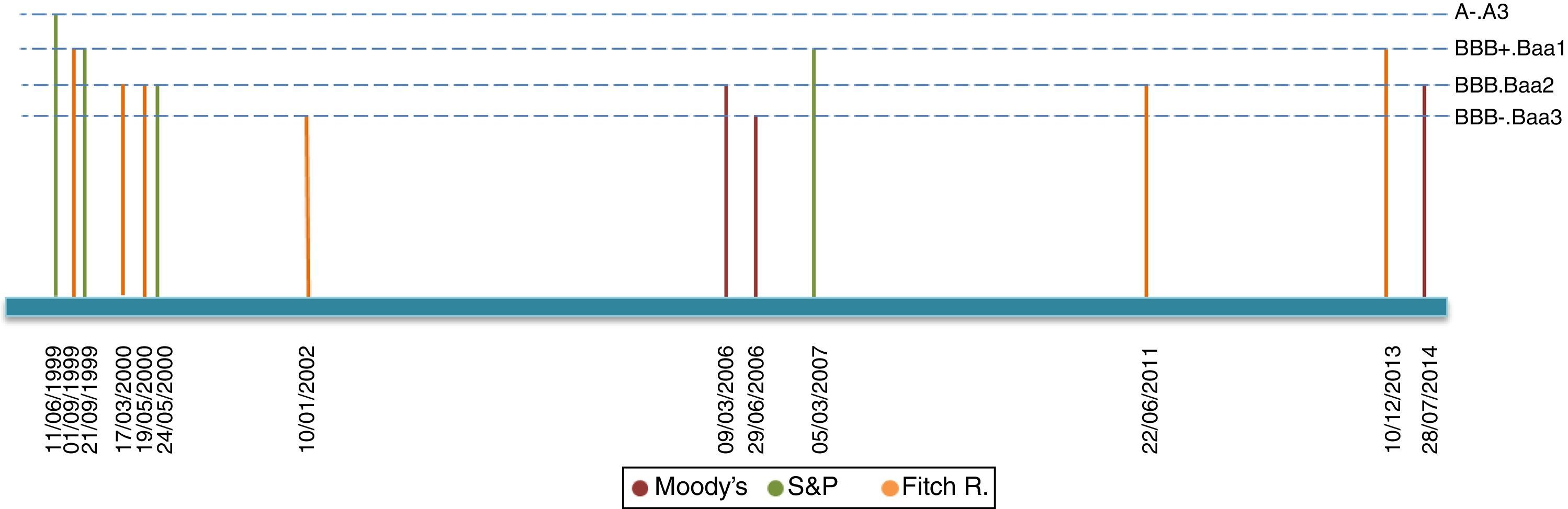
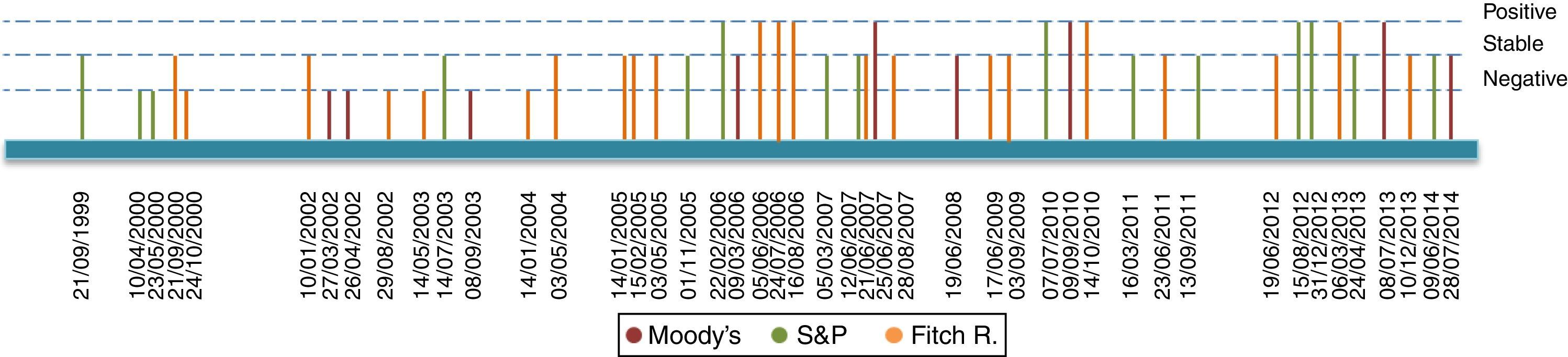
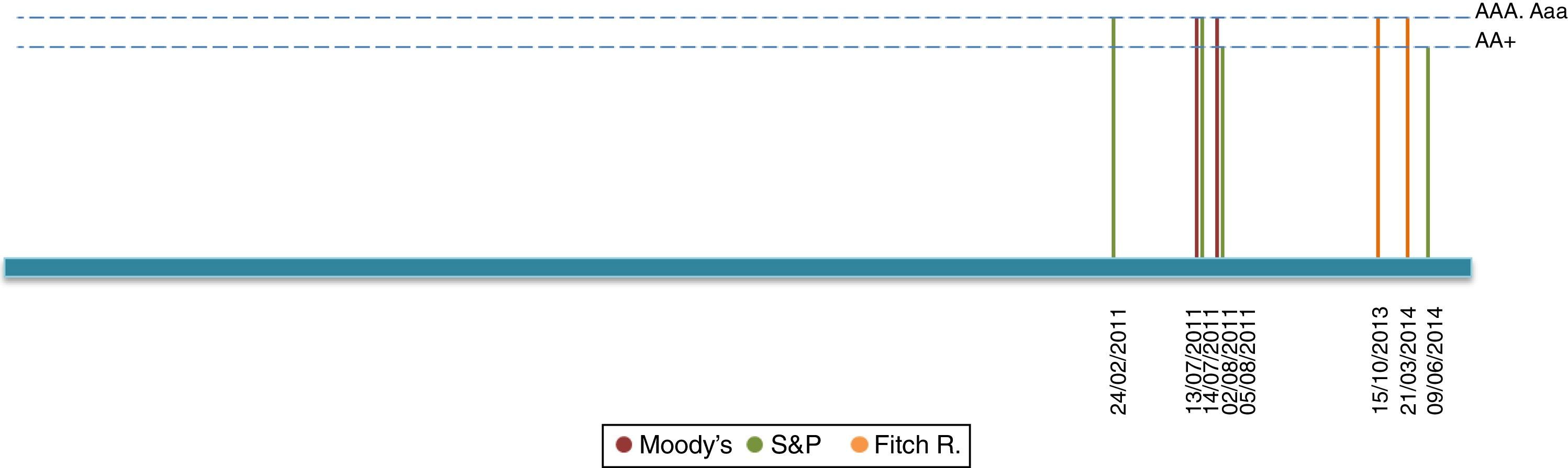
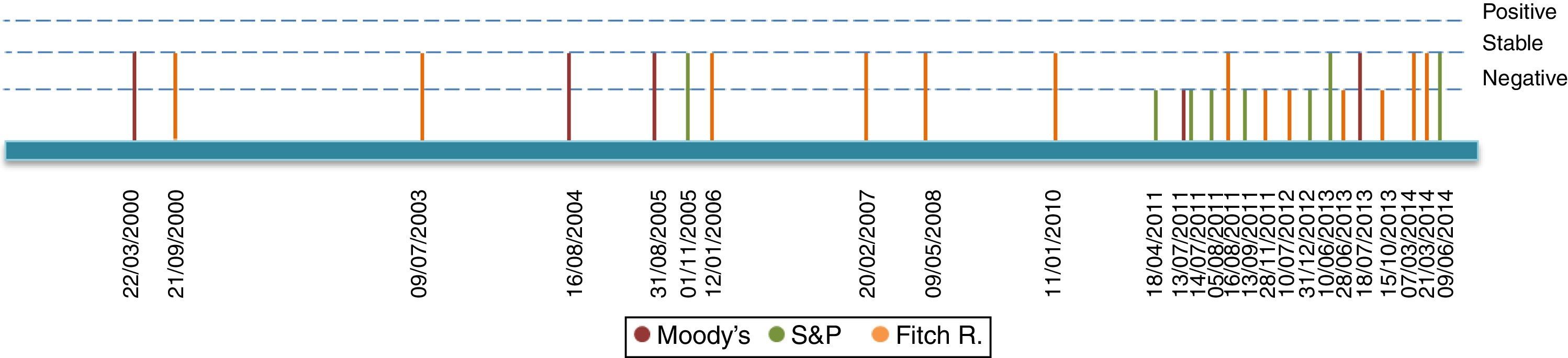
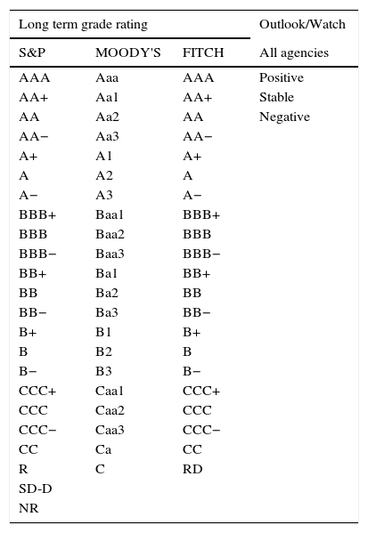
2Data description2.1Sovereign credit ratingsOur period of study dates from January 2003 up until September 2014. Our chosen rating agencies consist of Moody's, Standard and Poor's (S&P) and Fitch Ratings (Fitch). These agencies, which correspond to the most representative agencies in Colombia, provide two types of announcements concerning sovereign bonds: Outlook/Watch and Grade ratings. While the former imparts an overall perspective of the underlying asset structure, namely a Positive, Stable or Negative outlook, the latter indicates an agency-specific grade ranking. We present a list of each grade announcement (per agency) in Table A1 of Appendix A. Additionally, Table A5 of Appendix D describes the computation of events based on credit announcements.
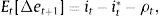
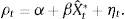
Figs. 1–4 depict announcements of long-term sovereign bonds (i.e. 1 and 5-year maturities) for both the United States and Colombia. Specifically, Figs. 2 and 4 depict Outlook/Watch announcements and Figs. 1 and 3 depict Grade ratings for the case of Colombia and the United States, respectively.
. Figure available in colour in the online version of the article.")
. Figure available in colour in the online version of the article.")
. Figure available in colour in the online version of the article.")
. Figure available in colour in the online version of the article.")
We employ two different portfolio measures in our estimations. Both are constructed with monthly data (of foreign and domestic bond holdings) obtained from the financial superintendency.3
Following Dominguez and Frankel (1993), our first measure (XDFp) consists of foreign (US) bond investments expressed in domestic currency, ¿tBt*, relative to total investment, as follows:
where Bt* and Bt denote foreign and domestic bonds, respectively, and ¿ is the nominal exchange rate expressed in Colombian Pesos per US dollar (COP/USD). The second measure (XRatp) is simply the ratio of foreign to domestic investment, expressed in units of domestic currency, as follows: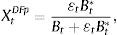

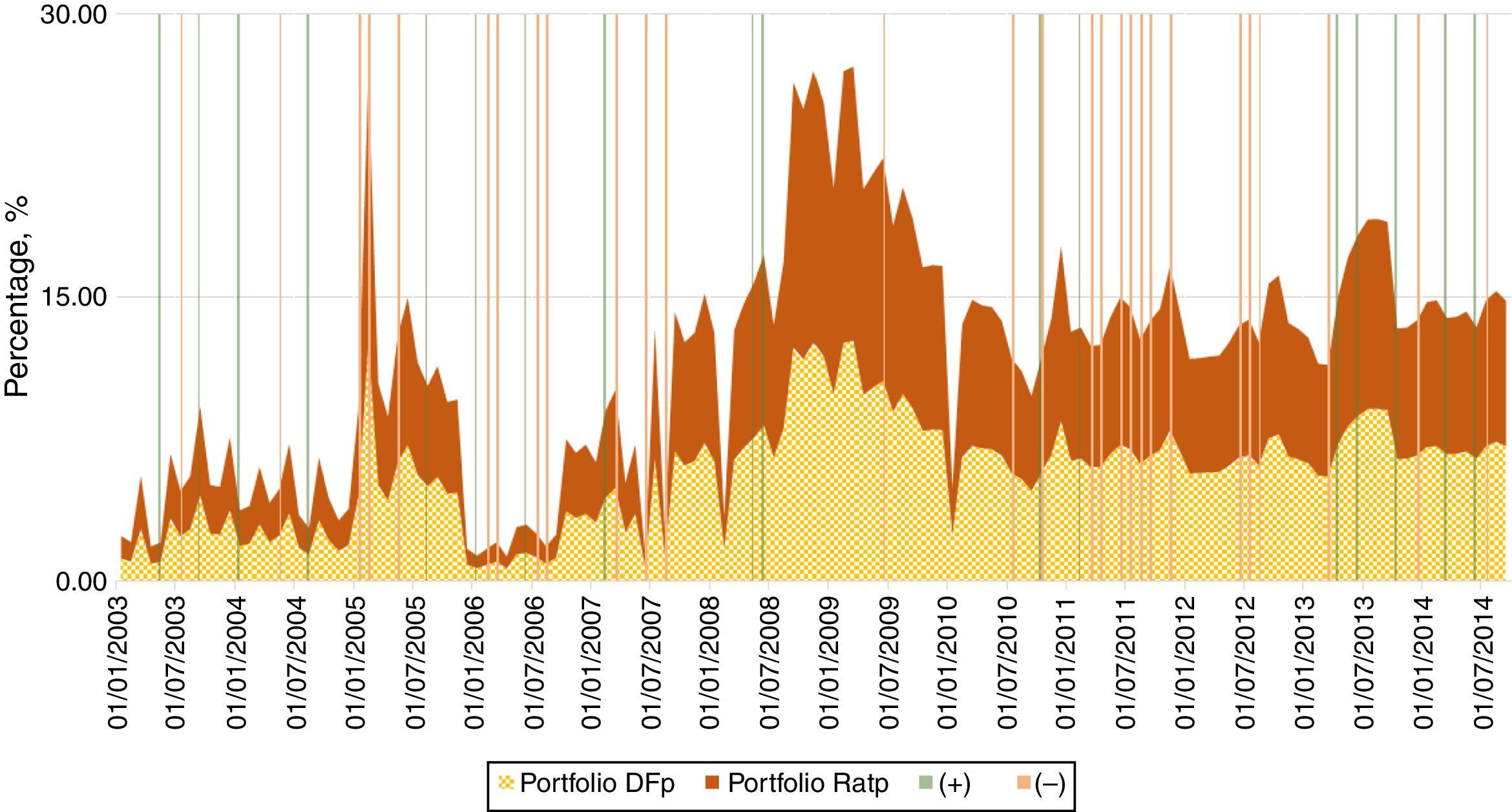
Fig. 5 depicts our two portfolio measures (i.e. total amount of domestic and foreign sovereign bond holdings) in the hands of the Colombian financial sector which amounts to all commercial banks, pension funds, and insurance companies. In particular, we show cases in which US ratings increased relative to Colombian ratings (“+” henceforth) and cases in which Colombian ratings increased relative to US ratings (“−” henceforth). To understand the portfolio's dynamics, we highlight two periods. First, in 2006 there was a drop in asset holdings of both dollar and pesos denominations. During that period, treasuries were highly valued commercial banks liquidated their positions to increase revenues. The second period is related to a more direct portfolio substitution towards foreign assets during 2008–2009 and a low substitution during 2003–2008. The heightened acceleration after 2006 was likely attributed to the high credit and liquidity risk preceding the financial world crisis.
2.3Other variables. Figure available in colour in the online version of the article.")
The remaining variables in our dataset are described as follows4:
- •
Variables used to estimate treatment effects on portfolio compositions
- –
Colombian Sovereign Bond (TES) Yields: Daily observations of treasury bond yields from the Central Bank of Colombia. Bond maturities of one and five years.
- –
US Sovereign Bond (T-BILL) Yields: Daily observations from the Federal Reserve of the United States. Bond maturities of one and five years.
- –
Exchange Rate Volatility (COP/USD): Daily observations from the Central Bank of Colombia, computed using an EWMA (Exponentially Weighted Moving Average). Other volatility measures using a GARCH(1,1) methodology and squared daily returns were also considered but not reported.
- –
WTI Crude Oil prices: Daily observations obtained from Bloomberg (USD per Barrel).
- –
Relative Output Growth: Difference between Colombian and US industrial production growth. Data from the Central Bank of Colombia and the Federal Reserve of the United States.
- –
- •
Variables used to compute departures from the UIP condition (i.e. risk premium)
- –
Exchange Rate (COP/USD): Daily average market rate from the Central Bank of Colombia.
- –
Expected Exchange Rate (COP/USD): Daily observations from the Central Bank of Colombia. We use two measures of expected exchange rates: the first measure consists of the one-year exchange rate forecasts from the expectations survey conducted monthly by the Central Bank of Colombia and covers the largest commercial banks, stockbrokers and pension funds in the country. The second measure is the one-year and five-year ahead ex-post exchange rate.
- –
Interest rate Differentials: Difference between US and Colombian sovereign bond yields.
- –
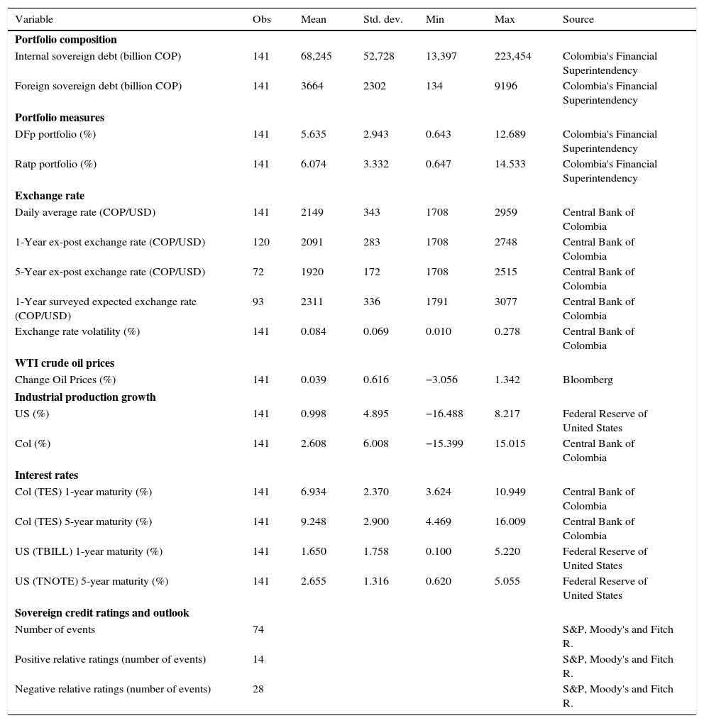
Finally, we present descriptive statistics for all variables in Table 1:
Descriptive statistics.
| Variable | Obs | Mean | Std. dev. | Min | Max | Source |
|---|---|---|---|---|---|---|
| Portfolio composition | ||||||
| Internal sovereign debt (billion COP) | 141 | 68,245 | 52,728 | 13,397 | 223,454 | Colombia's Financial Superintendency |
| Foreign sovereign debt (billion COP) | 141 | 3664 | 2302 | 134 | 9196 | Colombia's Financial Superintendency |
| Portfolio measures | ||||||
| DFp portfolio (%) | 141 | 5.635 | 2.943 | 0.643 | 12.689 | Colombia's Financial Superintendency |
| Ratp portfolio (%) | 141 | 6.074 | 3.332 | 0.647 | 14.533 | Colombia's Financial Superintendency |
| Exchange rate | ||||||
| Daily average rate (COP/USD) | 141 | 2149 | 343 | 1708 | 2959 | Central Bank of Colombia |
| 1-Year ex-post exchange rate (COP/USD) | 120 | 2091 | 283 | 1708 | 2748 | Central Bank of Colombia |
| 5-Year ex-post exchange rate (COP/USD) | 72 | 1920 | 172 | 1708 | 2515 | Central Bank of Colombia |
| 1-Year surveyed expected exchange rate (COP/USD) | 93 | 2311 | 336 | 1791 | 3077 | Central Bank of Colombia |
| Exchange rate volatility (%) | 141 | 0.084 | 0.069 | 0.010 | 0.278 | Central Bank of Colombia |
| WTI crude oil prices | ||||||
| Change Oil Prices (%) | 141 | 0.039 | 0.616 | −3.056 | 1.342 | Bloomberg |
| Industrial production growth | ||||||
| US (%) | 141 | 0.998 | 4.895 | −16.488 | 8.217 | Federal Reserve of United States |
| Col (%) | 141 | 2.608 | 6.008 | −15.399 | 15.015 | Central Bank of Colombia |
| Interest rates | ||||||
| Col (TES) 1-year maturity (%) | 141 | 6.934 | 2.370 | 3.624 | 10.949 | Central Bank of Colombia |
| Col (TES) 5-year maturity (%) | 141 | 9.248 | 2.900 | 4.469 | 16.009 | Central Bank of Colombia |
| US (TBILL) 1-year maturity (%) | 141 | 1.650 | 1.758 | 0.100 | 5.220 | Federal Reserve of United States |
| US (TNOTE) 5-year maturity (%) | 141 | 2.655 | 1.316 | 0.620 | 5.055 | Federal Reserve of United States |
| Sovereign credit ratings and outlook | ||||||
| Number of events | 74 | S&P, Moody's and Fitch R. | ||||
| Positive relative ratings (number of events) | 14 | S&P, Moody's and Fitch R. | ||||
| Negative relative ratings (number of events) | 28 | S&P, Moody's and Fitch R. | ||||
Authors’ calculations. Billion COP correspond to 109.
In this section, we provide a basic theoretical understanding of the portfolio balance channel by modeling how the banking sector optimally allocates its portfolio composition. This allows us to characterize departures from the UIP condition in terms of foreign and domestic assets. Formally, let the revenue of a given investment bank equal the return of investing in domestic and foreign sovereign bonds (B, B*). Following the corporate finance literature, we assume that banks are risk averse in terms of dividends (see Bianchi & Bigio, 2014, Allen & Michaely, 2003, Guttman, Kadan, & Kandel, 2010; Kumar & Spatt, 1987). Hence, a representative bank maximizes:
where Vt corresponds to the bank's dividend in period t, δtB and δtB* represent repayment probability rates (opposite to default rates) of domestic and foreign bonds, respectively, itB and itB* denote domestic and foreign bond yields, and ¿t is the nominal exchange rate expressed in units of domestic currency per unit of foreign currency. Additionally, we include a bond substitution cost function, Ψ(·), in order to allow bonds denominated in different currencies to be imperfect substitutes. For tractability purposes, we model this cost with a general CES representation: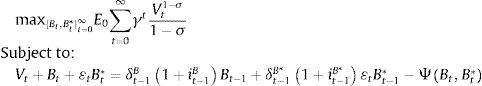

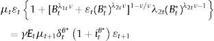
Intuitively, λiν≤1 corresponds to the substitution parameter between domestic and foreign bonds and captures the fact that some bonds are more liquid than others, possibly due to transaction costs (λ1 and λ2 represent liquidity parameters).
The model's adjustment cost function has important implications. First, as highlighted by Schmitt-Grohe and Uribe (2003), in an open economy with one international traded bond, the adjustment cost allows the interest rate to be determined by the total net asset position (in our case, the domestic interest rate depends endogenously on domestic and foreign assets). Second, liquidity frictions are introduced by having different degrees of substitutability (see Andres, López-Salido, & Nelson, 2004). Note that we do not explicitly model the interaction between credit ratings and investment decisions. Nevertheless, one possible channel is through the ratio between the repayment probabilities of domestic and foreign assets. That is, when this ratio increases, so does the interest rate spread and the expected depreciation. Accordingly, the optimality conditions with respect to domestic and foreign bonds yield:
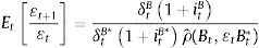
where μ is the Lagrange multiplier. Optimality conditions described in Eqs. (3.3) and (3.4) imply that inter-temporal marginal costs of dividends are compensated with marginal returns of each asset. Combining Eqs. (3.4) and (3.3) yields the Euler condition:where ρˆ(Bt,¿tBt*)=1+Btλ1tν+¿tBt*λ2tν1−ν/νλ1tBtλ1tν−11+Btλ1tν+¿tBt*λ2tν1−ν/νλ2tBt*λ2tν−1. As it turns out, Eq. (3.5) captures most of the intuition behind the UIP condition. Namely, expected exchange rate changes depend on interest rate differentials, relative repayment rates (i.e. country risk) and the risk premium. As stated in Villamizar-Villegas and Perez-Reyna (2015), the risk premium can be interpreted as the difference between a risk-free investment (foreign bond) and a risky investment (domestic bond) subject to unexpected exchange rate changes. As such, in the empirical exercise presented in Section 4, we use the following linear version of Eq. (3.5):where ρt=lnρˆ(Bt,¿tBt*)−ln(δtBδtB*) and et=ln(¿t). Note that Eq. (3.6) is the same equation used in Almekinders and Eijffinger (1996) and Kearns and Rigobon (2002).
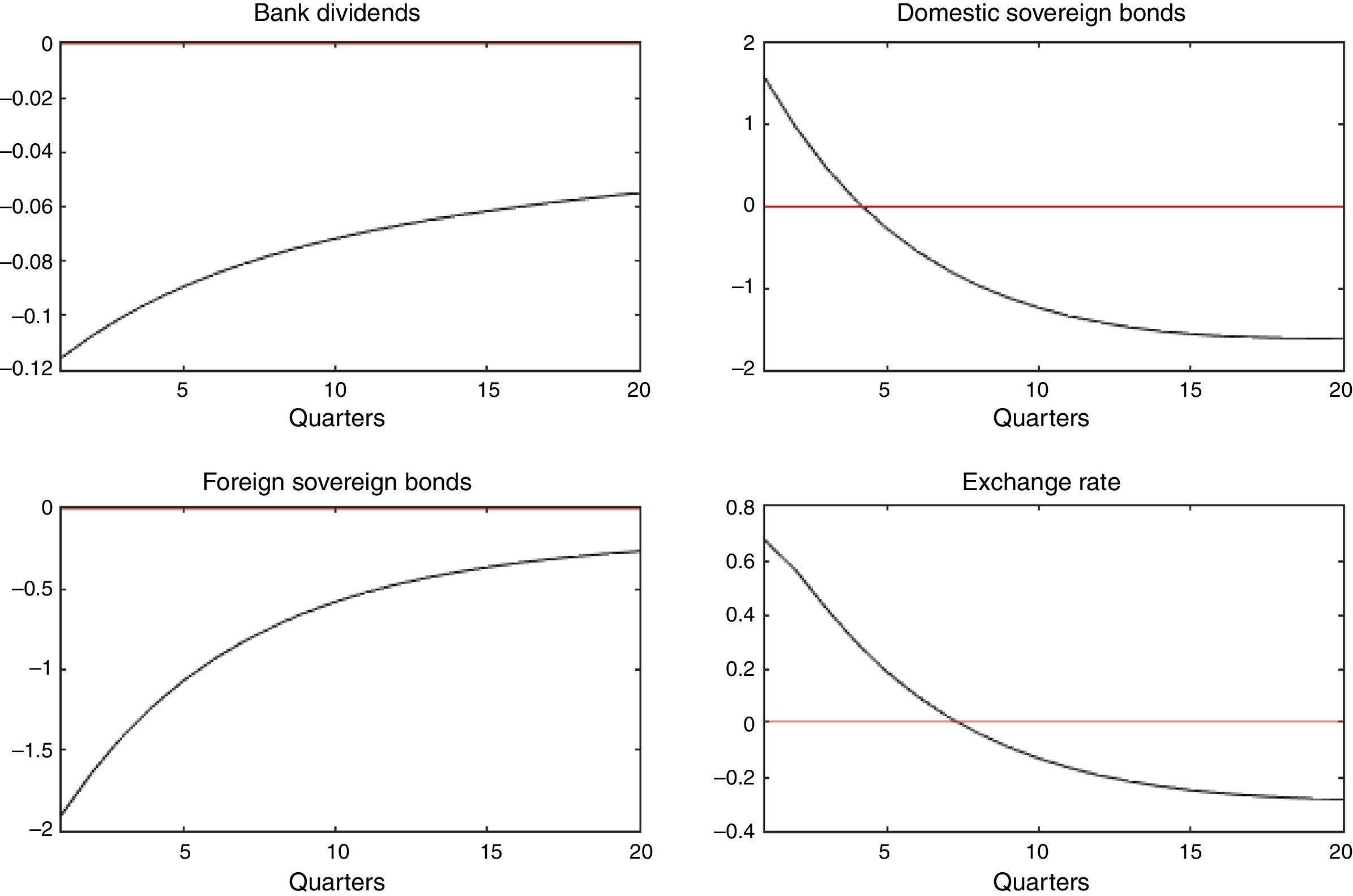
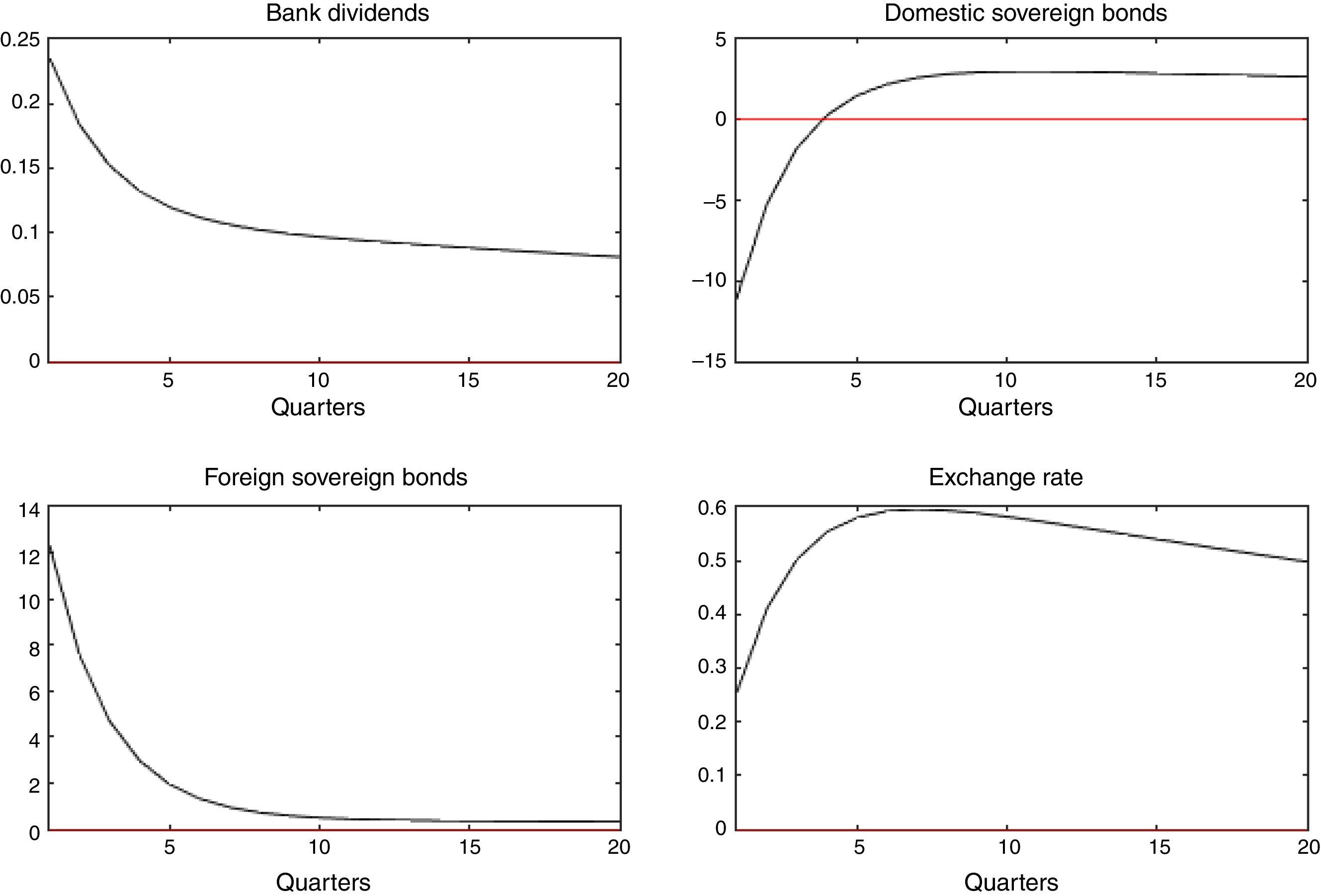
We finally characterize a partial equilibrium in this setup as a sequence of individual allocations {Vt,Bt,Bt*}t=0∞, and prices {itB,itB*,¿t}t=0∞, such that: (i) given {itB,itB*,¿t}t=0∞, and {δtB,δtB*}, the bank problem is solved and (ii) the sovereign bond market clears.5 To better understand the intuition behind Eq. (3.5), in Appendix B we compute and analyze Impulse Response Functions (IRFs) to shocks on liquidity and repayment rates.
4Empirical analysisConsistent with our theoretical framework, the first part of our methodology consists of estimating the effects of credit ratings on the Colombian portfolio composition, for which we use an event study analysis. We then study the effects of the estimated portfolio movements on departures from the UIP condition (i.e. risk premium).
Essentially, the main challenge of estimating portfolio effects is that they respond endogenously to factors which are correlated with the exchange rate. In the “selection on unobservables” literature, studies such as Dominguez and Frankel (1993) instrument portfolio changes with announcements on foreign exchange intervention so as to isolate effects driven by expectations. We believe, however, that even these intervention announcements might be subject to an endogenous relationship caused by exchange rate movements previous to the time of announcements.
We thus propose a novel instrument for shifts in the portfolio composition: the use of sovereign credit ratings. We argue that announcements on sovereign bonds largely affect investors’ decisions given that they reflect the ability of a government to meet its financial commitments. Moreover, we control for variables that are included in the glossaries of credit agencies and which are used as criteria for the computation of ratings. In this sense, we isolate portfolio movements from confounding effects (i.e. factors that concurrently affect the exchange rate).
4.1Calculating abnormal returns using an event study analysisAbnormal returns capture the main counterfactual of interest: what would have happened to portfolio balances if credit ratings had not changed, given that they did. Hence, they represent ideal candidates to test for variations in investment decisions which are as good as randomly assigned (at least with respect to factors that influence the exchange rate).
As such, we first identify all Outlook/Watch and Grade ratings within our sample from Moody's, Fitch and S&P that could potentially produce a change in investment decisions (see Section 2). Specifically, we identify cases in which US ratings increased relative to Colombian ratings (+) and in which Colombian ratings increased relative to US ratings (−). In order to appraise the event's impact on our selected portfolio measures, we compute abnormal returns (Xt*) defined as the difference between the observed ex-post value after each event (Xt) and the conditional mean of portfolio balances (Et[Xt|Ωt]), otherwise known as the normal return. Formally,
where Ωt denotes the conditioning information set at time t. Recall that we employ two different measures of portfolio balances (XtDFp and XtRatp), as described in Section 2.2.6
In order to estimate the normal return of Eq. (4.1), we first define an estimation window of [−13,−3] months (i.e. time period prior to each event) so as to control for variables that could have systematically affected portfolio balances. We then regress the following specification confined to the estimation window:
where Volt corresponds to exchange rate volatility, ΔOilt is the change in WTI oil prices, (it−itUS) is the yield differential between US and Colombian sovereign bonds, (Δyt−ΔytUS) is the relative industrial production growth between the United States and Colombia, and Devent is a Dummy variable which captures past events (i.e. past changes in relative credit ratings).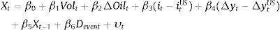
In essence, we include these control variables in order to avoid endogenous or anticipatory movements within our instrument (i.e. omitted variable bias). That is, we intend to identify exchange rate variations that are not attributed to changes in interest rate differentials (or factors that have an influence on interest rate differentials). For example, changes in oil prices can simultaneously affect the exchange rate and credit ratings, leading to an endogenous relationship (i.e. both Colombia and the United States are oil producing economies). Hence, our goal is to capture exogenous portfolio movements that are almost as good as randomly assigned. To this end, we employed variables published by credit agencies as glossaries of key indicators and which are used as criteria for the computation of ratings. This allows us to isolate movements within portfolio balance sheets that do not systematically react to several macroeconomic variables.
Normal returns are then computed by projecting Xt onto the event window (time period after the event). That is, we use the estimated coefficients obtained in Eq. (4.2) but use post-event values of covariates (see Campbell, Lo, & MacKinlay, 1996). Finally, in the last step of our methodology, we regress the risk premium on the estimated abnormal returns (Xˆt*) as follows:
It is in this final step where we benefit from the theoretical implications of our model. In particular, we assess whether abnormal returns of portfolio compositions have an effect on the risk premium (see Eq. (3.6)). Significant results would suggest that the risk premium is in fact a relevant driver through which the portfolio balance channel operates.
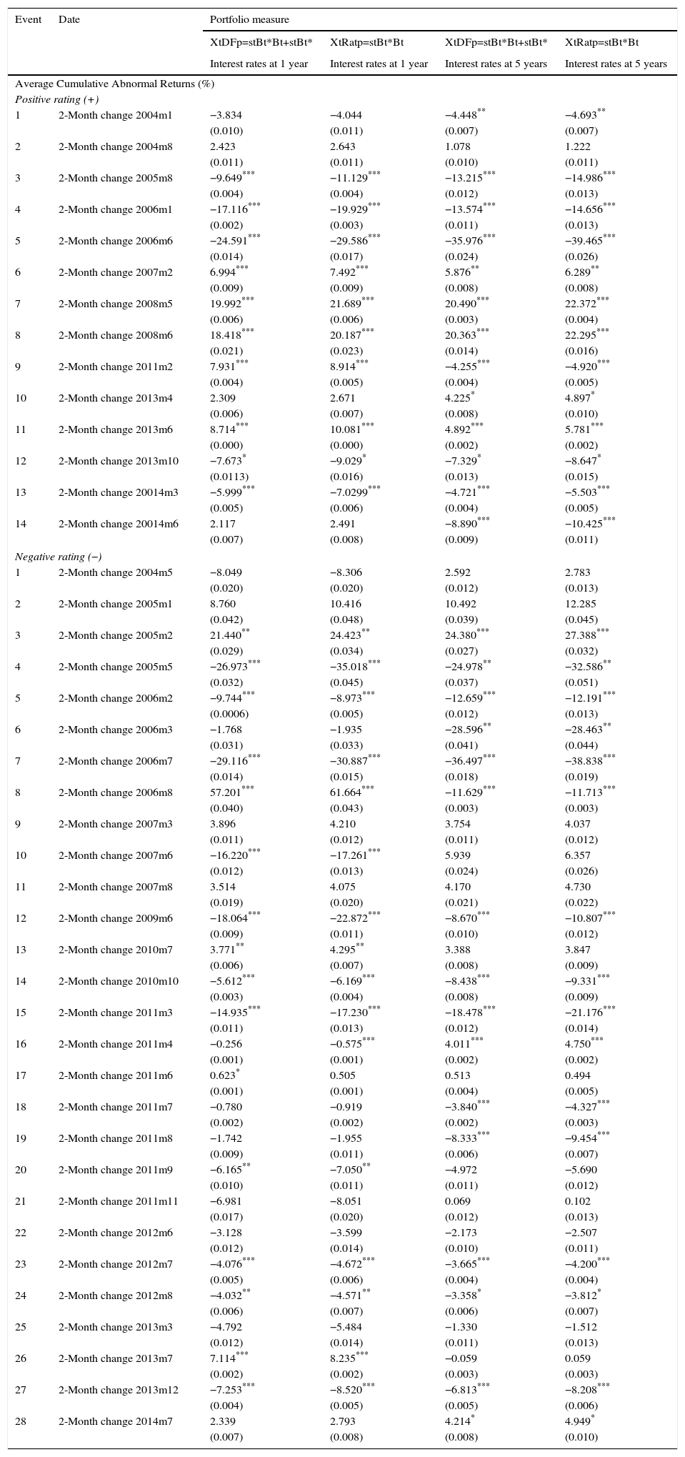
4.2ResultsResults are based on the average Cumulative Abnormal Returns (CAR) of Eq. (4.1) by using an estimation window of [−13,−3] months and an event window of [−1,1] months.7 As stated in the previous section, while the former allows us to control for episodes prior to the event, the latter is used for estimating abnormal returns.
Table 2 reports estimation results of Eq. (4.1) for the two portfolio measures: DFp and Ratp. Specifically, we report the one-sample t-test for the CAR of each event. We considered cases in which relative sovereign ratings increased (+) and decreased (−), as defined in Section 4.1. Additionally, we control for exchange rate volatility (measured as an Exponentially Weighted Moving Average – EWMA), changes in WTI oil prices, interest rate differentials between domestic and foreign bonds, relative output growth, and past credit ratings (see Eq. (4.2)).8
Effects of sovereign credit ratings on portfolio balances: Jan/2003–Sep/2014.
| Event | Date | Portfolio measure | |||
|---|---|---|---|---|---|
| XtDFp=stBt*Bt+stBt* | XtRatp=stBt*Bt | XtDFp=stBt*Bt+stBt* | XtRatp=stBt*Bt | ||
| Interest rates at 1 year | Interest rates at 1 year | Interest rates at 5 years | Interest rates at 5 years | ||
| Average Cumulative Abnormal Returns (%) | |||||
| Positive rating (+) | |||||
| 1 | 2-Month change 2004m1 | −3.834 | −4.044 | −4.448** | −4.693** |
| (0.010) | (0.011) | (0.007) | (0.007) | ||
| 2 | 2-Month change 2004m8 | 2.423 | 2.643 | 1.078 | 1.222 |
| (0.011) | (0.011) | (0.010) | (0.011) | ||
| 3 | 2-Month change 2005m8 | −9.649*** | −11.129*** | −13.215*** | −14.986*** |
| (0.004) | (0.004) | (0.012) | (0.013) | ||
| 4 | 2-Month change 2006m1 | −17.116*** | −19.929*** | −13.574*** | −14.656*** |
| (0.002) | (0.003) | (0.011) | (0.013) | ||
| 5 | 2-Month change 2006m6 | −24.591*** | −29.586*** | −35.976*** | −39.465*** |
| (0.014) | (0.017) | (0.024) | (0.026) | ||
| 6 | 2-Month change 2007m2 | 6.994*** | 7.492*** | 5.876** | 6.289** |
| (0.009) | (0.009) | (0.008) | (0.008) | ||
| 7 | 2-Month change 2008m5 | 19.992*** | 21.689*** | 20.490*** | 22.372*** |
| (0.006) | (0.006) | (0.003) | (0.004) | ||
| 8 | 2-Month change 2008m6 | 18.418*** | 20.187*** | 20.363*** | 22.295*** |
| (0.021) | (0.023) | (0.014) | (0.016) | ||
| 9 | 2-Month change 2011m2 | 7.931*** | 8.914*** | −4.255*** | −4.920*** |
| (0.004) | (0.005) | (0.004) | (0.005) | ||
| 10 | 2-Month change 2013m4 | 2.309 | 2.671 | 4.225* | 4.897* |
| (0.006) | (0.007) | (0.008) | (0.010) | ||
| 11 | 2-Month change 2013m6 | 8.714*** | 10.081*** | 4.892*** | 5.781*** |
| (0.000) | (0.000) | (0.002) | (0.002) | ||
| 12 | 2-Month change 2013m10 | −7.673* | −9.029* | −7.329* | −8.647* |
| (0.0113) | (0.016) | (0.013) | (0.015) | ||
| 13 | 2-Month change 20014m3 | −5.999*** | −7.0299*** | −4.721*** | −5.503*** |
| (0.005) | (0.006) | (0.004) | (0.005) | ||
| 14 | 2-Month change 20014m6 | 2.117 | 2.491 | −8.890*** | −10.425*** |
| (0.007) | (0.008) | (0.009) | (0.011) | ||
| Negative rating (−) | |||||
| 1 | 2-Month change 2004m5 | −8.049 | −8.306 | 2.592 | 2.783 |
| (0.020) | (0.020) | (0.012) | (0.013) | ||
| 2 | 2-Month change 2005m1 | 8.760 | 10.416 | 10.492 | 12.285 |
| (0.042) | (0.048) | (0.039) | (0.045) | ||
| 3 | 2-Month change 2005m2 | 21.440** | 24.423** | 24.380*** | 27.388*** |
| (0.029) | (0.034) | (0.027) | (0.032) | ||
| 4 | 2-Month change 2005m5 | −26.973*** | −35.018*** | −24.978** | −32.586** |
| (0.032) | (0.045) | (0.037) | (0.051) | ||
| 5 | 2-Month change 2006m2 | −9.744*** | −8.973*** | −12.659*** | −12.191*** |
| (0.0006) | (0.005) | (0.012) | (0.013) | ||
| 6 | 2-Month change 2006m3 | −1.768 | −1.935 | −28.596** | −28.463** |
| (0.031) | (0.033) | (0.041) | (0.044) | ||
| 7 | 2-Month change 2006m7 | −29.116*** | −30.887*** | −36.497*** | −38.838*** |
| (0.014) | (0.015) | (0.018) | (0.019) | ||
| 8 | 2-Month change 2006m8 | 57.201*** | 61.664*** | −11.629*** | −11.713*** |
| (0.040) | (0.043) | (0.003) | (0.003) | ||
| 9 | 2-Month change 2007m3 | 3.896 | 4.210 | 3.754 | 4.037 |
| (0.011) | (0.012) | (0.011) | (0.012) | ||
| 10 | 2-Month change 2007m6 | −16.220*** | −17.261*** | 5.939 | 6.357 |
| (0.012) | (0.013) | (0.024) | (0.026) | ||
| 11 | 2-Month change 2007m8 | 3.514 | 4.075 | 4.170 | 4.730 |
| (0.019) | (0.020) | (0.021) | (0.022) | ||
| 12 | 2-Month change 2009m6 | −18.064*** | −22.872*** | −8.670*** | −10.807*** |
| (0.009) | (0.011) | (0.010) | (0.012) | ||
| 13 | 2-Month change 2010m7 | 3.771** | 4.295** | 3.388 | 3.847 |
| (0.006) | (0.007) | (0.008) | (0.009) | ||
| 14 | 2-Month change 2010m10 | −5.612*** | −6.169*** | −8.438*** | −9.331*** |
| (0.003) | (0.004) | (0.008) | (0.009) | ||
| 15 | 2-Month change 2011m3 | −14.935*** | −17.230*** | −18.478*** | −21.176*** |
| (0.011) | (0.013) | (0.012) | (0.014) | ||
| 16 | 2-Month change 2011m4 | −0.256 | −0.575*** | 4.011*** | 4.750*** |
| (0.001) | (0.001) | (0.002) | (0.002) | ||
| 17 | 2-Month change 2011m6 | 0.623* | 0.505 | 0.513 | 0.494 |
| (0.001) | (0.001) | (0.004) | (0.005) | ||
| 18 | 2-Month change 2011m7 | −0.780 | −0.919 | −3.840*** | −4.327*** |
| (0.002) | (0.002) | (0.002) | (0.003) | ||
| 19 | 2-Month change 2011m8 | −1.742 | −1.955 | −8.333*** | −9.454*** |
| (0.009) | (0.011) | (0.006) | (0.007) | ||
| 20 | 2-Month change 2011m9 | −6.165** | −7.050** | −4.972 | −5.690 |
| (0.010) | (0.011) | (0.011) | (0.012) | ||
| 21 | 2-Month change 2011m11 | −6.981 | −8.051 | 0.069 | 0.102 |
| (0.017) | (0.020) | (0.012) | (0.013) | ||
| 22 | 2-Month change 2012m6 | −3.128 | −3.599 | −2.173 | −2.507 |
| (0.012) | (0.014) | (0.010) | (0.011) | ||
| 23 | 2-Month change 2012m7 | −4.076*** | −4.672*** | −3.665*** | −4.200*** |
| (0.005) | (0.006) | (0.004) | (0.004) | ||
| 24 | 2-Month change 2012m8 | −4.032** | −4.571** | −3.358* | −3.812* |
| (0.006) | (0.007) | (0.006) | (0.007) | ||
| 25 | 2-Month change 2013m3 | −4.792 | −5.484 | −1.330 | −1.512 |
| (0.012) | (0.014) | (0.011) | (0.013) | ||
| 26 | 2-Month change 2013m7 | 7.114*** | 8.235*** | −0.059 | 0.059 |
| (0.002) | (0.002) | (0.003) | (0.003) | ||
| 27 | 2-Month change 2013m12 | −7.253*** | −8.520*** | −6.813*** | −8.208*** |
| (0.004) | (0.005) | (0.005) | (0.006) | ||
| 28 | 2-Month change 2014m7 | 2.339 | 2.793 | 4.214* | 4.949* |
| (0.007) | (0.008) | (0.008) | (0.010) | ||
Source: Authors’ calculations. The table shows average Cumulative Abnormal Returns (CARs) using as control variables: exchange rate volatility, interest rate differentials, changes in oil prices, relative growth and past relative credit ratings (See Section 2). The first and third column refer to the Dominguez and Frankel (1993) portfolio measure, and the second and fourth column refer to the portfolio ratio (Ratp). We considered cases in which relative sovereign ratings increased (+) and decreased (−), as defined in Section 4.1. Standard errors are in parenthesis.
The resulting abnormal returns of Table 2 are robust (in significance and magnitude) across yield maturities of 1 and 5 years and across portfolio measures. In total, 33 out of 44 events were significant using 1-year bond maturities, and 27 out of 44 events were significant using 5-year bond maturities. Also, while positive (+) ratings led to both higher and lower portfolio balances, negative (−) ratings mostly led to a decrease in portfolio compositions (see Table 3). This last result, however, should be interpreted with caution given that abnormal returns are conditional on the set of control variables. In other words, the direction of portfolio shifts is obtained when accounting for movements in all covariates. Furthermore, we argue that unexpected signs of some events are due to the fact that foreign and domestic investors have different effects on the direction of change within portfolios. For example, while pension funds may increase their position of domestic assets after a negative event (e.g. after a US downgrade), foreign investor may also want to increase their domestic assets, by purchasing them from the financial sector. Given that we only have aggregated data for the entire financial sector, we refer the issue of differentiating capital flows within the financial sector to future research.
Summary of abnormal returns.
| Number of events | Positive and significant CAR | Negative and significant CAR | |
|---|---|---|---|
| Portfolio measures (DFp and Ratp) with 1-year maturity yields | |||
| (+) | 14 | 5 | 6 |
| (−) | 28 | 6 | 10 |
| Total | 42 | 11 | 16 |
| Portfolio measures (DFp and Ratp) with 5-year maturity yields | |||
| (+) | 14 | 5 | 9 |
| (−) | 28 | 4 | 13 |
| Total | 42 | 9 | 22 |
Source: Authors’ calculations. Cumulative Abnormal Returns are estimated by controlling for exchange rate volatility, interest rate differentials, changes in oil prices, relative output growth and past credit ratings for an event window of [−1,1] and an estimation window of [−13,−3]. A positive (negative) rating refers to the case in which US ratings increase (decrease) relative to Colombian ratings.
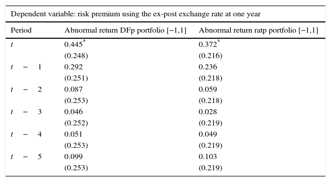
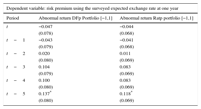
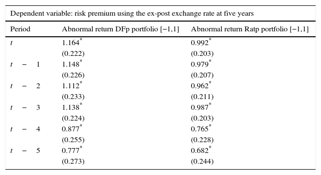
Tables 4–6 show results for the effects of the estimated abnormal returns on departures of UIP, as described by Eq. (4.3). Specifically, we use three measures of the risk premium which consist of: (i) the ex-post exchange rate at one year shown in Table 4, (ii) the surveyed expected exchange rate at one year shown in Table 5, and (iii) the ex-post exchange rate at five years shown in Table 6.
OLS estimation: ρt=α+βϵˆit*+ηt.
| Dependent variable: risk premium using the ex-post exchange rate at one year | ||
|---|---|---|
| Period | Abnormal return DFp portfolio [−1,1] | Abnormal return ratp portfolio [−1,1] |
| t | 0.445* | 0.372* |
| (0.248) | (0.216) | |
| t−1 | 0.292 | 0.236 |
| (0.251) | (0.218) | |
| t−2 | 0.087 | 0.059 |
| (0.253) | (0.218) | |
| t−3 | 0.046 | 0.028 |
| (0.252) | (0.219) | |
| t−4 | 0.051 | 0.049 |
| (0.253) | (0.219) | |
| t−5 | 0.099 | 0.103 |
| (0.253) | (0.219) | |
Source: Authors’ calculations. Abnormal returns are based on the Dominguez and Frankel (1993) (DFp) portfolio definition and on the portfolio ratio (Ratp). We control for exchange rate volatility, interest rate differentials, changes in oil prices, output growth and past relative credit ratings when a positive and a negative event occur with an event window of [−1,1] and an estimation window of [−13,−3]. Standard errors are reported in parenthesis.
OLS estimation: ρt=α+βϵˆit*+ηt.
| Dependent variable: risk premium using the surveyed expected exchange rate at one year | ||
|---|---|---|
| Period | Abnormal return DFp Portfolio [−1,1] | Abnormal return Ratp portfolio [−1,1] |
| t | −0.047 | −0.044 |
| (0.078) | (0.068) | |
| t−1 | −0.043 | −0.041 |
| (0.079) | (0.068) | |
| t−2 | 0.020 | 0.011 |
| (0.080) | (0.069) | |
| t−3 | 0.104 | 0.083 |
| (0.079) | (0.069) | |
| t−4 | 0.100 | 0.083 |
| (0.080) | (0.069) | |
| t−5 | 0.137* | 0.118* |
| (0.080) | (0.069) | |
Source: Authors’ calculations. Abnormal returns are based on the Dominguez and Frankel (1993) (DFp) portfolio definition and on the portfolio ratio (Ratp). We control for exchange rate volatility, interest rate differentials, changes in oil prices and output growth when a positive and a negative event occur with an event window of [−1,1] and an estimation window of [−13,−3]. Standard errors are reported in parenthesis.
OLS estimation: ρt=α+βϵˆit*+ηt.
| Dependent variable: risk premium using the ex-post exchange rate at five years | ||
|---|---|---|
| Period | Abnormal return DFp portfolio [−1,1] | Abnormal return Ratp portfolio [−1,1] |
| t | 1.164* | 0.992* |
| (0.222) | (0.203) | |
| t−1 | 1.148* | 0.979* |
| (0.226) | (0.207) | |
| t−2 | 1.112* | 0.962* |
| (0.233) | (0.211) | |
| t−3 | 1.138* | 0.987* |
| (0.224) | (0.203) | |
| t−4 | 0.877* | 0.765* |
| (0.255) | (0.228) | |
| t−5 | 0.777* | 0.682* |
| (0.273) | (0.244) | |
Source: Authors’ calculations. Abnormal returns are based on the Dominguez and Frankel (1993) (DFp) portfolio definition and on the portfolio ratio (Ratp). We control for exchange rate volatility, interest rate differentials, changes in oil prices and output growth when a positive and a negative event occur with an event window of [−1,1] and an estimation window of [−13,−3]. Standard errors are reported in parenthesis.
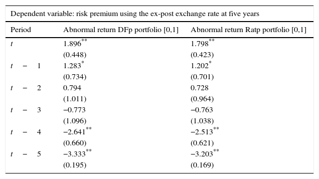
Results show that exchange rate effects are significant when considering departures from the UIP condition using 5-year exchange rate changes (Table 6). In fact, portfolio shifts (due to changes in credit ratings) increase the risk premium, as dictated by Eq. (3.6), in up to 5 months before the effects subside. This is not the case for the risk premium with a 1-year horizon, where effects are not statistically significant, except for the contemporary effect using the ex-post exchange rate (Table 4).9
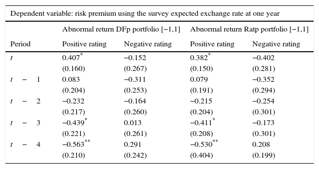
Additionally, Tables A9 and A10 of Appendix D show that, when estimating positive (+) and negative (−) ratings separately, the risk premium has a significant effect, especially after positive ratings. That is, the risk premium responds more to when US ratings increased relative to Colombian ratings than vice-versa.
A possible explanation of the stronger impact of portfolio balances in the long term relates to the intuition of investor's preferred habitat. As pointed out by Vayanos and Vila (2009), preferred habitats are relevant in order to study the maturity structure between different assets. Others explanations include regulatory and institutional constraints. In the case of Colombia for example, there are regulations on the amount of foreign holdings that affect investment decisions of the financial sector (see Cardozo et al., 2015).
5ConclusionsIn this paper we provide a theoretical understanding of the portfolio balance channel by extending the UIP to a case in which the banking sector optimally allocates its portfolio composition. In the empirical application, we propose a novel instrument for shifts in the portfolio composition: the use of relative credit ratings for US and Colombian sovereign bonds.
Our findings indicate that, when properly controlled for, shifts in portfolio balances affect the long term (5-year) risk premium, defined as departures from the UIP condition, in up to five months before the effects subside. Additionally, when separately considering cases in which US ratings increased (+) and decreased (−) relative to Colombian ratings, we find that the risk premium responds more to positive (+) ratings. The foregoing results show that not every credit rating change has a significant impact on agents’ asset allocations, but some announcements convey additional information which triggers a re-balancing of their financial portfolios.
Policy implications derived from this investigation are twofold. First, we find empirical evidence of the portfolio balance channel under certain time horizons. This potentially grants central banks an additional monetary tool to target the exchange rate without any alteration in the monetary base. Namely, if agents are risk-averse, then it is sufficient for shifts in the portfolio composition to have a direct effect on the exchange rate. Second, the fact that the risk premium responds more to positive than negative ratings opens up a line of research regarding financial and monetary policy, in which portfolio balances can be regulated depending on their asymmetric effects on capital flows.
We acknowledge the ample empirical literature that exists on both the effects of sovereign credit ratings and the exchange rate. However, only a handful of studies have addressed both and, to the best of our knowledge, there is no study that uses credit ratings as an instrument for the portfolio composition, outside of the present study. Consequently, we believe that our investigation will shed some light on the ongoing debate regarding both the theoretical and empirical effects of the portfolio balance channel.
Conflict of interestThe authors declare no conflict of interest.
Sovereign credit rating by agency.
| Long term grade rating | Outlook/Watch | ||
|---|---|---|---|
| S&P | MOODY'S | FITCH | All agencies |
| AAA | Aaa | AAA | Positive |
| AA+ | Aa1 | AA+ | Stable |
| AA | Aa2 | AA | Negative |
| AA− | Aa3 | AA− | |
| A+ | A1 | A+ | |
| A | A2 | A | |
| A− | A3 | A− | |
| BBB+ | Baa1 | BBB+ | |
| BBB | Baa2 | BBB | |
| BBB− | Baa3 | BBB− | |
| BB+ | Ba1 | BB+ | |
| BB | Ba2 | BB | |
| BB− | Ba3 | BB− | |
| B+ | B1 | B+ | |
| B | B2 | B | |
| B− | B3 | B− | |
| CCC+ | Caa1 | CCC+ | |
| CCC | Caa2 | CCC | |
| CCC− | Caa3 | CCC− | |
| CC | Ca | CC | |
| R | C | RD | |
| SD-D | |||
| NR | |||
Source: Standard and Poor's Services, Moody's Investors Service and Fitch Ratings.
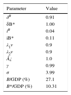
To better understand the intuition behind Eq. (3.5), we calibrate parameters as reported in Table A2. Namely, the model replicates the steady state ratio of domestic and foreign sovereign bonds with respect to the Colombian GDP during 2003–2014.
Parameters (quarterly).
| Parameter | Value |
|---|---|
| δB | 0.91 |
| δB* | 1.00 |
| iB | 0.04 |
| iB* | 0.11 |
| λ1ν | 0.9 |
| λ2ν | 0.9 |
| ¿ | 1.0 |
| γ | 0.99 |
| σ | 3.99 |
| B/GDP (%) | 27.1 |
| B*/GDP (%) | 10.31 |
Source: Authors’ calculations. Calibration based on quarterly frequency. Repayment probabilities are computed according to the findings of Peter (2002) for emerging economies. For the US, we assume a repayment probability equal to unity. The data source for the rest of variables is taken from the Colombian ministry of finance: The domestic interest rate corresponds to the Colombian sovereign bonds (TES-UVR), quarterly from 2003–2016 with a 5-year maturity. Foreign debt interest rate is computed as the weighted average between the medium and long term foreign debt for the period 2012–2015. Domestic and foreign bonds (quarterly) are computed as a ratio of GDP (%) for the period 2003–2014. The risk aversion and discounting factor are taken from the DSGE literature applied to the Colombian economy (see González, Mahadeva, Prada, & Rodríguez, 2011). λ1ν and λ2ν are ad-hoc imposed.
Additionally, we assume that shocks on domestic liquidity and repayment rates follow auto-regressive processes exemplified by (B.1) and (B.2):
and further assume that ηt, ζt∼N(0, σ2). Next, IRFs are computed to a one standard deviation shock in ηt and ζt.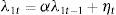
Fig. 6 depicts the response of bank's dividends, domestic and foreign sovereign bonds, and the exchange rate, to a domestic liquidity shock (ηt). Results are in line with the portfolio channel (see Weber, 1986) and show that the exchange rate depreciates given a higher demand for domestic bond holdings and a lesser demand for foreign bonds.1010 The opposite is true after considering a foreign liquidity shock.
. Figure available in colour in the online version of the article.")

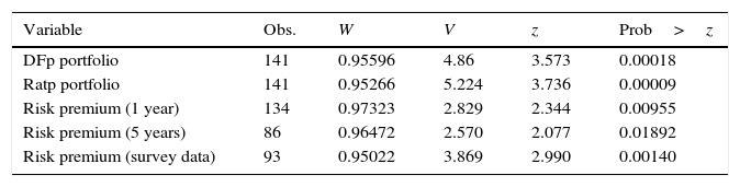
Normality test 2003–2014 (Shapiro–Wilk W test).
| Variable | Obs. | W | V | z | Prob>z |
|---|---|---|---|---|---|
| DFp portfolio | 141 | 0.95596 | 4.86 | 3.573 | 0.00018 |
| Ratp portfolio | 141 | 0.95266 | 5.224 | 3.736 | 0.00009 |
| Risk premium (1 year) | 134 | 0.97323 | 2.829 | 2.344 | 0.00955 |
| Risk premium (5 years) | 86 | 0.96472 | 2.570 | 2.077 | 0.01892 |
| Risk premium (survey data) | 93 | 0.95022 | 3.869 | 2.990 | 0.00140 |
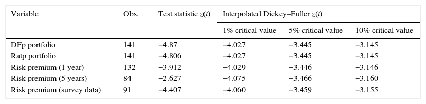
Dickey–Fuller unit root test.
| Variable | Obs. | Test statistic z(t) | Interpolated Dickey–Fuller z(t) | ||
|---|---|---|---|---|---|
| 1% critical value | 5% critical value | 10% critical value | |||
| DFp portfolio | 141 | −4.87 | −4.027 | −3.445 | −3.145 |
| Ratp portfolio | 141 | −4.806 | −4.027 | −3.445 | −3.145 |
| Risk premium (1 year) | 132 | −3.912 | −4.029 | −3.446 | −3.146 |
| Risk premium (5 years) | 84 | −2.627 | −4.075 | −3.466 | −3.160 |
| Risk premium (survey data) | 91 | −4.407 | −4.060 | −3.459 | −3.155 |
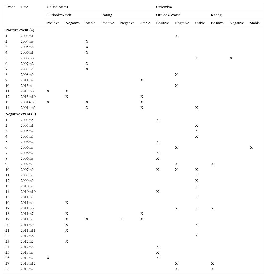
Relative events: Jan/2003–Sep/2014.
| Event | Date | United States | Colombia | ||||||||||
|---|---|---|---|---|---|---|---|---|---|---|---|---|---|
| Outlook/Watch | Rating | Outlook/Watch | Rating | ||||||||||
| Positive | Negative | Stable | Positive | Negative | Stable | Positive | Negative | Stable | Positive | Negative | Stable | ||
| Positive event (+) | |||||||||||||
| 1 | 2004m1 | X | |||||||||||
| 2 | 2004m8 | X | |||||||||||
| 3 | 2005m8 | X | |||||||||||
| 4 | 2006m1 | X | |||||||||||
| 5 | 2006m6 | X | X | ||||||||||
| 6 | 2007m2 | X | |||||||||||
| 7 | 2008m5 | X | |||||||||||
| 8 | 2008m6 | X | |||||||||||
| 9 | 2011m2 | X | |||||||||||
| 10 | 2013m4 | X | |||||||||||
| 11 | 2013m6 | X | X | ||||||||||
| 12 | 2013m10 | X | X | ||||||||||
| 13 | 20014m3 | X | X | X | |||||||||
| 14 | 20014m6 | X | X | X | |||||||||
| Negative event (−) | |||||||||||||
| 1 | 2004m5 | X | |||||||||||
| 2 | 2005m1 | X | |||||||||||
| 3 | 2005m2 | X | |||||||||||
| 4 | 2005m5 | X | |||||||||||
| 5 | 2006m2 | X | |||||||||||
| 6 | 2006m3 | X | X | ||||||||||
| 7 | 2006m7 | X | |||||||||||
| 8 | 2006m8 | X | |||||||||||
| 9 | 2007m3 | X | X | ||||||||||
| 10 | 2007m6 | X | X | X | |||||||||
| 11 | 2007m8 | X | |||||||||||
| 12 | 2009m6 | X | |||||||||||
| 13 | 2010m7 | X | |||||||||||
| 14 | 2010m10 | X | |||||||||||
| 15 | 2011m3 | X | |||||||||||
| 16 | 2011m4 | X | |||||||||||
| 17 | 2011m6 | X | X | X | |||||||||
| 18 | 2011m7 | X | X | ||||||||||
| 19 | 2011m8 | X | X | X | X | ||||||||
| 20 | 2011m9 | X | X | ||||||||||
| 21 | 2011m11 | X | |||||||||||
| 22 | 2012m6 | X | |||||||||||
| 23 | 2012m7 | X | |||||||||||
| 24 | 2012m8 | X | |||||||||||
| 25 | 2013m3 | X | |||||||||||
| 26 | 2013m7 | X | X | ||||||||||
| 27 | 2013m12 | X | X | ||||||||||
| 28 | 2014m7 | X | X | ||||||||||
Source: Authors’ calculations. In the event of multiple announcements per month, we assigned the following values, to serve as tie-breakers: Positive Change on Rating=1, Negative Change on Rating=−1, Same Rating Report=0.2, Positive Change on Outlook=0.5, Negative Change on Outlook=−0.5, Outlook report remains Stable=0.05, Outlook report remains Positive=0.1, and Outlook report remains Negative=−0.1.
Thus, the sign of the sum (per month) determines if an event is positive or negative (see Section 2).
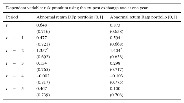
OLS estimation: ρt=α+βϵˆit*+ηt.
| Dependent variable: risk premium using the ex-post exchange rate at one year | ||
|---|---|---|
| Period | Abnormal return DFp portfolio [0,1] | Abnormal return Ratp portfolio [0,1] |
| t | 0.648 | 0.873 |
| (0.716) | (0.658) | |
| t−1 | 0.477 | 0.594 |
| (0.721) | (0.668) | |
| t−2 | 1.357* | 1.404* |
| (0.692) | (0.638) | |
| t−3 | 0.134 | 0.298 |
| (0.765) | (0.717) | |
| t−4 | −0.002 | −0.103 |
| (0.817) | (0.775) | |
| t−5 | 0.467 | 0.100 |
| (0.739) | (0.708) | |
Source: Authors’ calculations. Abnormal returns are based on the Dominguez and Frankel (1993) (DFp) portfolio definition and on the portfolio ratio (Ratp). We control for exchange rate volatility, interest rate differentials, changes in oil prices, output growth and past relative credit ratings when a positive and a negative event occur with an event window of [0,1] and an estimation window of [−13,−3]. Standard errors are reported in parenthesis.
OLS estimation: ρt=α+βϵˆit*+ηt.
| Dependent variable: risk premium using the surveyed expected exchange rate at one year | ||
|---|---|---|
| Period | Abnormal return DFp portfolio [0,1] | Abnormal return Ratp portfolio [0,1] |
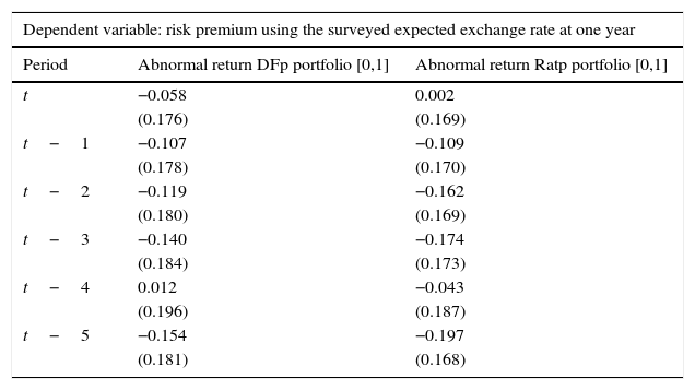
| t | −0.058 | 0.002 |
| (0.176) | (0.169) | |
| t−1 | −0.107 | −0.109 |
| (0.178) | (0.170) | |
| t−2 | −0.119 | −0.162 |
| (0.180) | (0.169) | |
| t−3 | −0.140 | −0.174 |
| (0.184) | (0.173) | |
| t−4 | 0.012 | −0.043 |
| (0.196) | (0.187) | |
| t−5 | −0.154 | −0.197 |
| (0.181) | (0.168) | |
Source: Authors’ calculations. Abnormal returns are based on the Dominguez and Frankel (1993) (DFp) portfolio definition and on the portfolio ratio (Ratp). We control for exchange rate volatility, interest rate differentials, changes in oil prices and output growth when a positive and a negative event occur with an event window of [0,1] and an estimation window of [−13,−3]. Standard errors are reported in parenthesis.
OLS estimation: ρt=α+βϵˆit*+ηt.
| Dependent variable: risk premium using the ex-post exchange rate at five years | ||
|---|---|---|
| Period | Abnormal return DFp portfolio [0,1] | Abnormal return Ratp portfolio [0,1] |
| t | 1.896** | 1.798** |
| (0.448) | (0.423) | |
| t−1 | 1.283* | 1.202* |
| (0.734) | (0.701) | |
| t−2 | 0.794 | 0.728 |
| (1.011) | (0.964) | |
| t−3 | −0.773 | −0.763 |
| (1.096) | (1.038) | |
| t−4 | −2.641** | −2.513** |
| (0.660) | (0.621) | |
| t−5 | −3.333** | −3.203** |
| (0.195) | (0.169) | |
Source: Authors’ calculations. Abnormal returns are based on the Dominguez and Frankel (1993) (DFp) portfolio definition and on the portfolio ratio (Ratp). We control for exchange rate volatility, interest rate differentials, changes in oil prices and output growth when a positive and a negative event occur with an event window of [0,1] and an estimation window of [−13,−3]. Standard errors are reported in parenthesis.
OLS estimation: ρt=α+βϵˆit*+ηt.
| Dependent variable: risk premium using the ex-post exchange rate at one year | ||||
|---|---|---|---|---|
| Abnormal return DFp portfolio [−1,1] | Abnormal return Ratp portfolio [−1,1] | |||
| Period | Positive rating | Negative rating | Positive rating | Negative rating |
| t | 2.532** | 1.681** | 2.291** | 1.524** |
| (0.744) | (0.461) | (0.673) | (0.419) | |
| t−1 | 3.127** | 1.052* | 2.822** | 0.935 |
| (0.646) | (0.530) | (0.586) | (0.483) | |
| t−2 | 2.650** | 0.630 | 2.406** | 0.537 |
| (0.794) | (0.550) | (0.719) | (0.501) | |
| t−3 | 2.488** | 0.514 | 2.257** | 0.420 |
| (0.874) | (0.548) | (0.793) | (0.499) | |
| t−4 | 0.543 | 0.829 | 0.490 | 0.711 |
| (0.070) | (0.545) | (0.972) | (0.498) | |
Source: Authors’ calculations. Abnormal Returns are based on the Dominguez and Frankel (1993) (DFp) portfolio definition and on the portfolio ratio (Ratp). We control for exchange rate volatility, interest rate differentials, changes in oil prices and output growth when a positive and a negative event occur with an event window of [−1,1] and an estimation window of [−13,−3]. Standard errors are reported in parenthesis.
OLS estimation: ρt=α+βϵˆit*+ηt.
| Dependent variable: risk premium using the survey expected exchange rate at one year | ||||
|---|---|---|---|---|
| Abnormal return DFp portfolio [−1,1] | Abnormal return Ratp portfolio [−1,1] | |||
| Period | Positive rating | Negative rating | Positive rating | Negative rating |
| t | 0.407* | −0.152 | 0.382* | −0.402 |
| (0.160) | (0.267) | (0.150) | (0.281) | |
| t−1 | 0.083 | −0.311 | 0.079 | −0.352 |
| (0.204) | (0.253) | (0.191) | (0.294) | |
| t−2 | −0.232 | −0.164 | −0.215 | −0.254 |
| (0.217) | (0.260) | (0.204) | (0.301) | |
| t−3 | −0.439* | 0.013 | −0.411* | −0.173 |
| (0.221) | (0.261) | (0.208) | (0.301) | |
| t−4 | −0.563** | 0.291 | −0.530** | 0.208 |
| (0.210) | (0.242) | (0.404) | (0.199) | |
Source: Authors’ calculations. Abnormal Returns are based on the Dominguez and Frankel (1993) (DFp) portfolio definition and on the portfolio ratio (Ratp). We control for exchange rate volatility, interest rate differentials, changes in oil prices and output growth when a positive and a negative event occur with an event window of [−1,1] and an estimation window of [−13,−3]. Standard Errors are reported in parenthesis.
Theoretical surveys that provide an in-depth view of the portfolio balance channel include Sarno and Taylor (2001), Evans (2005), Lyons (2006), and Villamizar-Villegas and Perez-Reyna (2015).
We are grateful Pamela Cardozo and Hernando Vargas and two anonymous referees for valuable feedback. The views expressed herein are those of the authors and not necessarily those of the Banco de la República nor its Board of Directors.
Studies that directly evaluate the impact of credit ratings on the exchange rate, without explicitly examining the portfolio balance channel include Alsakka and Ap Gwilym (2012), Treepongkaruna and Wu (2012), and Bissoondoyal-Bheenick et al. (2011). Alternatively, studies that center on the portfolio balance channel include Dominguez and Frankel (1993), Edison (1993), Dominguez (2003), Fatum and Hutchison (2003), Neely (2005), Menkhoff (2010), Villamizar-Villegas and Perez-Reyna (2015), Cardozo, Gamboa, Perez-Reyna, and Villamizar-Villegas (2015), and Kuersteiner, Phillips, and Villamizar-Villegas (2016).
Data were obtained from the Superintendencia Financiera de Colombia. See Table 1 for a summary of descriptive statistics.
Median values were considered for variables with a daily and weekly frequency in order to match with the financial sector data. Normality tests and stationarity properties are reported in Tables A3 and A4 of Appendix C.
If we assume a continuum of bonds B(s) for s∈(0, 1), then the market clearing condition implies that ∫01(Bt+¿tBt*)dF(s)=0.
In the finance literature, the normal return compares the return of any given security to the return of the market portfolio. In our case, we assume a linear specification which follows from assuming a joint-normal distribution of asset returns.
Results using event windows of [−2,2] and [−3,3] (not reported) yield similar results.
Other volatility measures, using a GARCH(1,1) methodology and squared daily returns (not reported) were employed but not reported, with similar results.
Tables A6–A8 show similar exercises as those presented in Tables 4–6 but now considering a 1-month event window of [0,1] and excluding credit reports that confirmed the previous agency's report. As shown, results are very similar.