External debt and monetary policy autonomy

Abstract

During a time of rising world interest rates, the central bank of a small open economy may be motivated to increase its own interest rate to keep from suffering a destabilizing outflow of capital and depreciation in the exchange rate. Empirically, this paper shows that this is especially true for a small open economy with a current account deficit, which relies on foreign capital inflows to finance this deficit. In addition, the method of current account financing has a large effect on whether or not the central bank will opt for exchange rate and capital flow stabilization during a time of rising world interest rates. A current account deficit financed mainly through reserve depletion or the accumulation of private sector debt will cause the central bank to pursue de facto exchange rate stabilization, whereas a current account deficit financed through equity or FDI will not. Quantitatively, reserve depletion of about 7% of GDP will motivate the central bank with a floating currency to adjust its interest rate in line with the foreign interest rate to where it appears that the central bank has an exchange rate peg.

Resumen

Durante un periodo de tasas de interés mundiales al alza, el banco central de una economía abierta pequeña podría verse motivado a aumentar su tasa de interés para evitar sufrir una salida de capital desestabilizadora y una depreciación de la tasa de cambio. El presente artículo muestra de manera empírica que esto es especialmente cierto para una economía abierta pequeña con un déficit en cuenta corriente, la cual depende de la entrada de capital extranjero para financiar su déficit. Asimismo, el método de financiación de cuenta corriente tiene un efecto importante sobre si el banco central optará o no por la estabilización de la tasa del cambio y flujo de capital durante un periodo de alza de tasa de interés mundial. Un déficit de cuenta corriente financiado fundamentalmente con el agotamiento de la reserva o la acumulación de deuda procedente del sector privado ocasionará que el banco central busque de facto la estabilización de la tasa de cambio, mientras que un déficit de cuenta corriente que se financie mediante la venta de acciones o inversión extranjera directa no lo hará. Desde el punto de vista cuantitativo, un agotamiento de la reserva de un 7% del PIB motivará que el banco central con moneda flotante ajuste su tasa de interés en línea con la tasa de interés extranjera con la que parezca que el banco central tiene fijado un tipo de cambio.

1

Introduction

In 2015, the Banco de México, the central bank in Mexico, rescheduled their monetary policy meetings to occur immediately following the meetings of the Federal Reserve. Monetary policy makers in Mexico knew that Fed lift-off from near-zero interest rate policy was imminent, and they wanted to arrange it such that the Banco de México could lift-off from their own extraordinarily low interest rates as soon as the Fed moved, and thus prevent a sudden shift in capital flows that would result in a sharp depreciation in the peso. When the Fed increased interest rates by 25 basis points on December 16th, the Banco de México matched them with a similar 25 basis point increase on December 17th.

The tendency for a central bank to mimic the monetary actions of a base currency central bank like the Federal Reserve is well documented. Usually the intention is to forestall a shift in capital flows that would lead to a sharp appreciation or depreciation of the currency. As shown in Shambaugh (2004), Obstfeld, Shambaugh, and Taylor (2005), and Klein and Shambaugh (2015), a way to measure monetary policy autonomy in the data is to regress changes in the policy interest rate in one country on changes in a base country interest rate. These papers find that the coefficient in this regression is much higher in countries with a pegged currency than in those with a floating currency, and the coefficient is higher for a country with an open capital account than in a country with a closed capital account.

In a country with a pegged exchange rate and an open capital account this need to match monetary policy actions is automatic, as implied by the famous trilemma from Mundell (1963) and Fleming (1962). By the same logic, monetary policy autonomy is automatic in a country with a floating exchange rate. Mechanically, a central bank with a floating currency has complete monetary policy autonomy and can do whatever it likes with its interest rate. But if the central bank has complete monetary policy autonomy, they can always choose to mimic a base country interest rate, and thus adopt a de facto exchange rate peg or soft peg. This paper will ask how a country's net external liability position might affect the central bank's choice of whether to pursue a monetary policy based solely on domestic concerns like the output gap or inflation, adopt a de facto exchange rate peg in an attempt to manage their external accounts.

Using a regression framework similar to that in Klein and Shambaugh (2015), we find that central banks in countries with a worsening external liability position (a current account deficit) are likely to move their interest rate in concert with a base country interest rate, and thus adopt some sort of de facto currency peg in an attempt to manage the external account. The intuition is as follows. A current account deficit needs to be financed by a positive net inflow of capital. An interest rate increase in the base country means that foreign investments are more attractive, and this leads to the possibility that those capital flows would reverse. As a result, central banks in countries with a current account deficit would find it necessary to raise their interest rate in order to retain foreign capital that would be tempted to flee.

A number of authors question the degree of monetary policy autonomy in a country with a floating exchange rate that is subject to exogenous swings in capital inflows and outflows (see e.g. Rey, 2015). Obstfeld (2015) discusses how financial globalization affects the trade-offs faced by monetary policy makers. Edwards (2015) examines the case of three Latin American countries with flexible exchange rates, inflation targeting and capital mobility and finds evidence that these countries tend to mimic Federal Reserve policy, and thus the degree of monetary policy autonomy is lower than would be expected. Dąbrowski, Śmiech, and Papież (2015) argue that ex-ante exchange rate regimes do not fully predetermine monetary policy response to shocks. They liken this to a “fear of floating” (Calvo & Reinhart, 2002) or more specifically, a “fear of losing international reserves” (Aizenman & Hutchison, 2012; Aizenman & Sun, 2012).

Forbes and Klein (2015) look at policy responses to a stop in capital inflows, and raising interest rates is one of them. But they argue that among possible policy options, raising interest rates leads to a sharp drop in GDP and is definitely not the most favorable option. Other options include reserve depletion, allowing the currency to depreciate, or imposing capital controls. However, reserve depletion may not be an option for a country with already depleted reserves, currency depreciation may not be favorable in a country with a large stock of foreign currency denominated debt, and temporary episodic capital controls may be difficult to implement in practice.¹ Intuitively, we find that not all forms of external liability accumulation cause a central bank to opt away from monetary policy autonomy toward a de facto peg. Only a currency account deficit financed by reserve depletion or the accumulation of foreign currency denominated debt cause a central bank to willingly sacrifice monetary policy autonomy. Equity financing or domestic currency denominated debt do not have the same effect.

These results are based on regressions that end in 2011. But the “taper tantrum” episode of the summer of 2013 provides a nice out-of-sample example of the mechanisms involved in this paper. Eichengreen and Gupta (2014), Mishra, Moriyama, and N’Diaye (2014), and Shaghil, Coulibaly, and Zlate (2015) all find that economic fundamentals like the current account had an effect on relative performance among emerging markets during the taper tantrum. Countries that ran a large current account deficit prior to the summer of 2013 were most adversely affected during the summer of 2013. Although Aizenman, Binici, and Hutchison (2014) find the opposite. In line with the subject of this paper, Arteta, Kose, Ohnsorge, and Stocker (2015) argue that economic fundaments were important part of the policy response to the taper tantrum. In the next section we will show how the emerging markets with current account deficits were the ones that were most likely to raise interest rates after the first suggestion of Fed tapering. Furthermore, the difference in interest rate responses across emerging markets is due to cross-country differences in debt-based capital inflows. Emerging markets that prior to the announcement of tapering received positive net debt inflows saw a much greater increase in rates than those with negative net debt inflows. Whether a country had positive or negative net equity inflows prior to 2013 had no effect on the subsequent interest rate response.

This paper will proceed as follows. The out-of-sample example of comparing policy responses across emerging markets during the “taper tantrum” is presented in Section 2. The formal econometric model and data that is used to measure the effect of external debt accumulation on monetary policy autonomy is presented in Section 3. The econometric results as well as the results from various robustness checks are presented in Section 4. Finally, Section 5 concludes.

2

Emerging market policy interest rates during the “taper tantrum”

In congressional testimony in May 2013, then Fed chairman Ben Bernanke first suggested that the Fed may begin to curtail the large scale asset purchase program known as QE3. This suggestion sent shock-waves through the international markets as the suggestion of tapering was interpreted to mean that the days of extraordinarily loose monetary policy in the U.S. were soon to come to an end.

Many believed that this monetary policy had led to a surge of capital inflows into many emerging market countries in a search for yield. This surge in capital inflows led to a sharp appreciation in currency and asset values. The reasoning went that the end of this extraordinary monetary policy accommodation by the Federal Reserve would lead to a reversal of those capital flows, and thus a sharp drop in currency and asset values across the emerging world. Investors would be smart to sell their emerging market assets now, ahead of Fed action; this itself led to a wave of capital outflows and triggered a sort of a crisis in many emerging markets in the summer of 2013 that has come to be known as the “taper tantrum”.

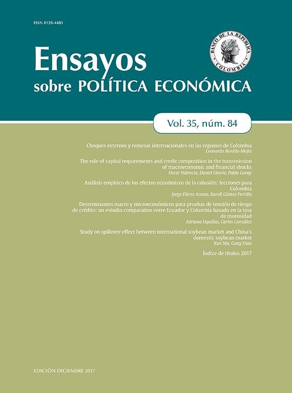
In a bid to attract or retain capital which was now fleeing in the expectation of higher interest rates in the U.S., many emerging market central banks raised their interest rates following the tapering announcement. The path of the GDP weighted average of policy interest rates across many emerging markets is shown in the green dotted line in the top panel of Fig. 1.² The vertical dotted line in the chart marks May 2013, when Chairman Bernanke first mentioned tapering. The chart shows that the late spring of 2013 marked the end of a two year easing cycle across emerging markets that began in the summer of 2011. In the year following the May 2013 announcement, emerging market policy rates increased by an average of 80 basis points.

Fig. 1.

Policy rates in emerging market economies with a current account deficit or surplus, positive or negative net debt inflows, and positive or negative net equity inflows. The red dashed line represents those with a current account deficit or positive net capital inflows and the blue solid line represents those with a current account surplus or negative net capital inflows.

But this average masks considerable heterogeneity in monetary tightening across the emerging markets. Countries with a current account deficit tightened quickly and tightened sharply. In the chart in the top panel of Fig. 1, the average among countries with a current account deficit is represented by the red dashed line and that for countries with a current account surplus is shown with the blue solid line. In the year following the tapering announcement, emerging markets with a current account deficit raised their policy rate by an average of 137 basis points while those with a current account surplus raised their policy rate by an average of 25 basis points.

In the late summer of 2013, some of these emerging market countries with a current account deficit were dubbed the “fragile five”, the large emerging market countries with current account deficits (Brazil, Indonesia, India, Turkey, and South Africa). A current account deficit needs to be financed by a positive net inflow of capital. The expectation of monetary policy normalization in the U.S. led to the possibility that those capital flows would reverse. As a result, central banks in countries with a current account deficit found it necessary to raise interest rates in order to retain foreign capital that would be tempted to flee.

2.1

Are all forms of deficit financing the same?

The current account is simply the negative of net capital inflows. Thus a country with a current account deficit must have positive net capital inflows. But these capital inflows can come in many forms. Capital inflows can be equity based, like FDI or portfolio equity, or they could be based on debt, like bank lending, portfolio debt, or central bank reserves.

Equity based capital inflows tend to be a much more stable form of financing than debt based capital inflows. Milesi-Ferretti and Tille (2011) and Lane and Milesi-Ferretti (2012) show that bank loans and other types of debt-based capital flows have seen the largest swings over the past few years. Forbes and Warnock (2014) show that debt based capital flows are more susceptible to episodes of stop or flight.³ In the taper tantrum of 2013 central banks in countries with a current account deficit found it necessary to raise their interest rates in order to retain these capital flows. But this fear of capital flight should apply to countries that were financing this deficit through debt inflows, not countries that depend on equity capital inflows.

Furthermore, equity based capital inflows tend to be home currency denominated, whereas in most emerging market countries, most debt based capital inflows tend to be denominated in a foreign currency like the U.S. dollar. McKinnon and Schnabl (2004a, 2004b) discuss the importance of having a high stock of foreign currency denominated assets for exchange rate stabilization. Countries without a high stock of foreign currency denominated assets, like U.S. dollar foreign exchange reserves, are more likely to turn to interest rate changes in order to stabilize the exchange rate.

The middle panel in Fig. 1 plots the path of the policy interest rate in emerging markets, but whereas before these policy rates were plotted for the group of countries with a current account deficit and those with a current account surplus, here they are plotted for the group of countries with positive net debt inflows and negative net debt inflows. The average among countries with positive net debt inflows is represented by the red dashed line and that for countries with negative net debt inflows is shown with the blue solid line.

Those with positive net debt inflows were countries that at the time of Bernanke's tapering announcement were relying on foreign debt inflows. The chart shows that central banks in those countries sharply tightened policy immediately after the tapering announcement, but central banks in countries with negative net debt inflows did not. In the year following the tapering announcement, central banks in countries with positive net debt inflows raised interest rates by an average of 165 basis points, central banks in the other set of countries lowered interest rates by an average of 10 basis points over the same year.

If instead we divide this group of emerging market countries into those with positive net equity inflows and those with negative net equity inflows, this strong dichotomy disappears. This is plotted in the bottom panel in Fig. 1, where the average policy interest rate among countries with positive net equity inflows is represented by the red dashed line and that for countries with negative net equity inflows is shown with the blue solid line. Countries with positive net equity inflows relied on inflows of foreign capital, but since this capital was based on equity and not debt, there was much less fear of capital flight. In the year following the tapering announcement, countries with positive equity inflows raised their policy interest rates by an average of 84 basis points, while countries with negative equity inflows raised rates by an average of 58 basis points.

The large spike in policy rates in late 2014 for countries with negative net equity inflows is entirely due to Russia, which raised interest rates by 750 basis points in December 2014. Russia had a current account surplus in 2014, and thus was exporting capital to the rest of the world. But the central bank was forced to act so dramatically in late 2014 due to a sharp fall in foreign exchange reserves due to the falling price of oil, the main Russia export, and the effects of sanctions placed on Russia in response to the situation in the Ukraine. Thus the Russian experience in late 2014 provides the textbook example of how a central bank faced with rapid reserve depletion may opt to increase the policy interest rate to curtail capital flight.

3

Econometric model and data

The econometric specification we use in the estimations begins with the familiar uncovered interest parity condition:

where S_t is the nominal exchange rate (in units of country i currency per units of the base country b currency), R_it is the country i nominal interest rate, Ritb is the base country nominal interest rate, and ¿_it is a risk premium. All variables are in log form.

If a central bank wants to stabilize their exchange rate, they should keep R_it close to Ritb+¿it.

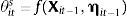
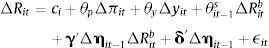
The central bank in country i follows the following monetary policy rule⁴:

where R¯it is the natural (Wicksellian) nominal rate of interest, π_it is inflation over the past year, π¯i is the central bank's inflation target, y_it is the log level of real GDP, y¯it is the log level of potential real GDP, and m_t is a monetary policy shock. The central bank's weights on the inflation and output gaps are given by θ_p and θ_y, respectively, and θits is the weight that the central places on exchange rate stabilization. We assume that θits is a function of a vector of institutional characteristics and the country's net external asset position:

where η_it−1 is a vector of the country's net external assets at the end of the last period. For our purposes, η_it−1 is a vector with 5 rows, the first is domestic currency denominated net external debt assets, the second is foreign currency denominated net external debt assets, the third is net external FDI assets, the fourth is net external portfolio equity assets, and the fifth is central bank foreign exchange reserves.

The vector X_it−1 contains all the variables that might affect a central bank's preference for exchange rate stabilization that are unrelated to the country's net external asset position, η_it−1. Variables in the vector X_it−1 include things like institutional characteristics that might affect central bank credibility, the extent of capital controls in the country, and a country's openness to trade and their trading partners. This paper will rely on first differences for identification, and thus many of the institutional characteristics in X_it will not appear in the differences regression. Vegh and Vuletin (2012) show how these institutional characteristics affect a central bank's preference for exchange rate stability. Furthermore, capital controls many appear in X_it. But capital control measures like the Chinn-Ito index tend to be very persistent from one year to the next. Klein and Shambaugh (2015) argue that “gates” type capital controls, those that change from one year to the next, tend not to be very effective in controlling capital flows, and Fernández et al. (2015) show that capital controls tend to be acyclical, an indication that policy makers are not using capital controls as a policy instrument to controls capital flows over the cycle.

So while the variables in X_it are very important for determining a country's preference for exchange rate stabilization, they tend not to move very much from year to year. So the change in θits from one year to the next is given by:

where the vector γ is simply the vector of first derivatives of the function f with respect to η_it. Thus the vector γ measures how a country's net external asset position might affect their preference for exchange rate stabilization.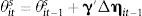

The vector γ can either have the same entry in each row, in which case γ′Δη_it−1 is simply equal to a constant γ multiplied by the change in a country's net external asset position (which is approximately equal to the current account). If γ < 0 then in response to a current account deficit that needs to be financed by foreign capital inflows, the central bank will increase the weight they put on exchange rate stabilization in their policy rule. Alternatively the entries in the vector γ may vary, indicating that changes in some types of net external liabilities affect the central bank's preference for exchange rate stabilization more than others.

So after taking the first difference of the Taylor rule policy function:

where ci=R¯it−R¯it−1−y¯it+y¯it−1. After a few substitutions this becomes:

3.1

Data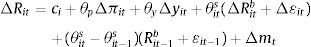

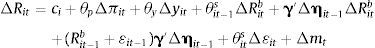
The expression in (5) can be estimated to identify the terms in the vector γ, the vector that measures how a country's net external asset position might affect their preference for exchange rate stabilization. Considering that the risk premium term in the UIP condition, ¿_it is not observable, the expression lends itself to the following reduced form empirical specification:

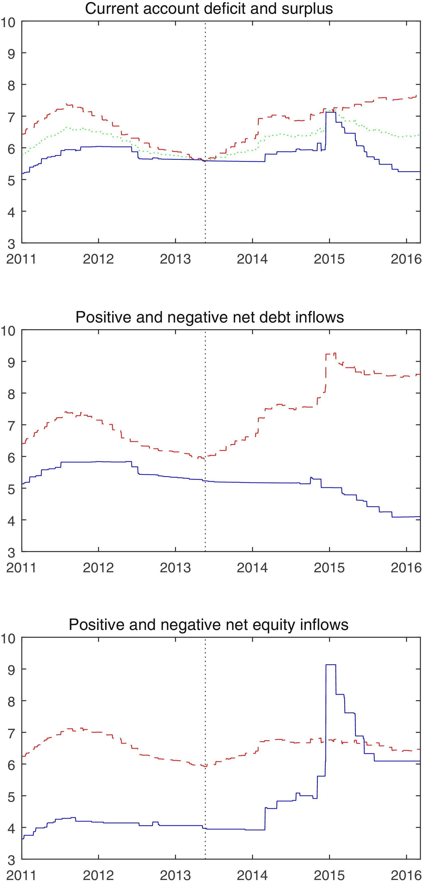
The two terms ΔR_it and ΔRitb are simply the year-over-year change in the country i's nominal interest rate and the base country nominal interest rate. In this estimation we consider an unbalanced panel consisting of 96 countries and 20 years, 1992–2011. The base country will vary across countries and years. The list of the 96 countries and their corresponding base country are presented in Table 1. The base country currency is the U.S. Dollar for 60% of the countries in the sample, the German Mark/euro for 27%, the French Franc/euro for 11%, and one each for the Australian Dollar, Indian Rupee, and Malaysian Ringgit. Klein and Shambaugh (2015) assemble this data in an unbalanced panel including 132 countries over the years 1973–2011. Because of data availability when constructing variables for foreign and domestic currency denominated external debt, we are forced to limit the sample. By dropping the need to separately estimate the effects of domestic and foreign currency denominated debt, we can expand the sample to the sample used in Klein and Shambaugh (2015). This wider sample does not affect the results and this robustness check is presented in the last section.

Table 1.

Countries in the sample and their corresponding base country.

Country name	Base country	Country name	Base country
United Kingdom	Germany	Benin	France
Austria	Germany	Ethiopia	United States
Belgium	Germany	Madagascar	France
Denmark	Germany	Malawi	United States
France	Germany	Mali	France
Germany	United States	Mozambique	United States
Italy	Germany	Niger	France
Netherlands	Germany	Nigeria	United States
Norway	Germany	Rwanda	United States
Sweden	Germany	Senegal	France
Switzerland	Germany	Fiji	United States
Canada	United States	Papua New Guinea	United States
Japan	United States	Azerbaijan	United States
Finland	Germany	Albania	Germany
Greece	Germany	Slovak Republic	Germany
Iceland	Germany	Israel	United States
Ireland	Germany	Turkey	United States
Portugal	Germany	South Africa	United States
Spain	Germany	Argentina	United States
Australia	United States	Brazil	United States
New Zealand	Australia	Chile	United States
Bolivia	United States	Colombia	United States
Dominican Republic	United States	Mexico	United States
El Salvador	United States	Peru	United States
Guatemala	United States	Venezuela	United States
Paraguay	United States	Jordan	United States
Uruguay	United States	Egypt	United States
Jamaica	United States	Hong Kong, China	United States
Oman	United States	India	United States
Yemen	United States	Indonesia	United States
Sri Lanka	India	Korea	United States
Ghana	United States	Malaysia	United States
Cote d’Ivoire	France	Pakistan	United States
Kenya	United States	Philippines	United States
Tanzania	United States	Singapore	Malaysia
Togo	France	Thailand	United States
Tunusia	France	Vietnam	United States
Uganda	United States	Algeria	France
Burkina Faso	France	Morocco	France
Zambia	United States	Armenia	United States
Georgia	United States	Russia	United States
Kazakhistan	United States	Ukraine	United States
Kyrgyz Republic	United States	Czech Republic	Germany
Moldova	United States	Estonia	Germany
Latvia	United States	Hungary	Germany
Slovenia	Germany	Lithuania	Germany
Romania	Germany	Croatia	Germany
Trinidad and Tobago	United States	Poland	Germany

The two variables Δπ_it and Δy_it are simply the year-over-year change in CPI inflation rate and log real GDP.

As discussed earlier, the vector η_it−1 contains five terms, domestic currency denominated net external debt assets, foreign currency denominated net external debt assets, net external FDI assets, net external portfolio equity assets, and central bank reserve assets at the end of the previous year.⁵ Most of this data is taken from the external wealth of nations dataset from Lane and Milesi-Ferretti (2007). The Share of external debt assets and liabilities that are denominated in the domestic or foreign currency is taken from Bénétrix, Lane, and Shambaugh (2015).

Before estimating this equation, it is helpful (but not necessary) to give some functional form to θit−1s. As discussed earlier, Klein and Shambaugh (2015) show that θst−1i is a function of whether or not a country has a pegged currency and the extent of capital controls. Klein and Shambaugh (2015) divide the country-year observations in their sample into those countries with a de facto exchange rate peg (where over the course of the year, a country's exchange rate relative to the base country never strays from within a ±2% band), those with a de facto soft peg (where the band is greater than ±2% but less than ±5%), and those with a floating currency (those that do not have a de facto peg or soft peg). In addition, the extent of capital account openness may be an important component of θit−1s. Therefore, when presenting the estimation results, we will first consider the case where θit−1s is a constant to be estimated, and alternatively we will consider the case where θit−1s takes the following form:

where peg_it−1 and soft_it−1 are indicator variables equal to 1 if the country-year observation has a pegged currency or a soft peg (as defined by Klein and Shambaugh (2015)) and K_it is simply the Chinn and Ito (2008) capital account openness index for that country-year observation (the original index is then normalized on a 0–1 scale where 0 denotes a closed capital account and 1 denotes an open capital account).

Of course a high-comovement between movements in the home and base country interest rate, captured by a high value for θits, could represent (1) the effort by the central bank to stabilize the exchange rate and capital flows, or (2) the home country and the base country reacting similarly to a common shock. This paper of course is trying to emphasize the first channel, but the second is still a possibility. By controlling for the normal Taylor rule variables inflation and the output gap, the risk of the results being driven by the common shock is mitigated. If the central banks of both the home and base countries were reacting to a common shock, and this shock were orthogonal to domestic inflation and the output gap, then the omission of the common shock from the regression would lead to an upward bias on the coefficient on the base country interest rate. However, in reality the risk of there being a common shock that is orthogonal to domestic inflation and the output gap is small, so the risk of this omitted variable bias is small.

The caveat to the regression in (6) is the potential endogeneity of the change in inflation term and the output growth term, both of which enter the regression equation as contemporaneous variables. But while these variables are potentially endogenous, the base country interest rate is exogenous. So this potential endogeneity may lead to a bias on the estimated coefficients on inflation and the output gap, but the coefficient on the base country interest rate will be consistent. In addition, the net foreign asset variable in the functional form for θits is lagged one period. This is specifically to address possible endogeneity in this variable. The contemporaneous net external asset variable may be endogenous to the current state of monetary policy, but one can assume that last year's external asset variable is not. Thus the interactions between the base country interest rate and these lagged net external asset variables are also exogenous, and the estimated values the terms in the vector γ are consistent. Potential endogeneity would only affect the coefficients on the output gap and inflation, but these variables are included as a control, nothing more.

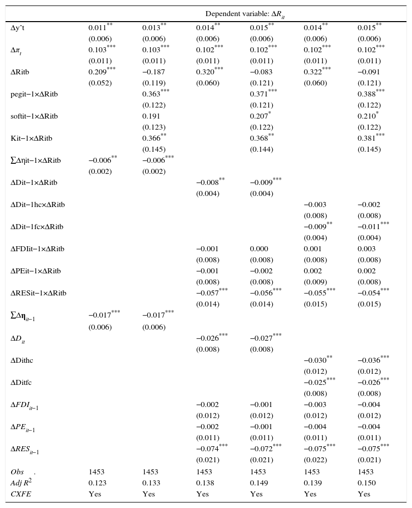
4

Results

The baseline regression results are presented in Table 2. The first two columns present the results from the regression where instead of estimating the effect of each component of the change in the international investment position, Δη_it−1, separately, we simply sum the components. The estimate of the interaction between ∑Δη_it−1 and changes in the foreign interest rate is the estimated value of γ in Eq. (6), where because we are treating each component of the vector Δη_it−1 equally, the coefficient vector γ is simply a scalar γ multiplied by a vector of ones. In this estimated value of the scalar γ is approximately equal to −0.006.

Table 2.

Benchmark regression results.

	Dependent variable: ΔRit
Δyˆt	0.011^**	0.013^**	0.014^**	0.015^**	0.014^**	0.015^**
	(0.006)	(0.006)	(0.006)	(0.006)	(0.006)	(0.006)
Δπt	0.103^***	0.103^***	0.102^***	0.102^***	0.102^***	0.102^***
	(0.011)	(0.011)	(0.011)	(0.011)	(0.011)	(0.011)
ΔRitb	0.209^***	−0.187	0.320^***	−0.083	0.322^***	−0.091
	(0.052)	(0.119)	(0.060)	(0.121)	(0.060)	(0.121)
pegit−1×ΔRitb		0.363^***		0.371^***		0.388^***
		(0.122)		(0.121)		(0.122)
softit−1×ΔRitb		0.191		0.207^*		0.210^*
		(0.123)		(0.122)		(0.122)
Kit−1×ΔRitb		0.366^**		0.368^**		0.381^***
		(0.145)		(0.144)		(0.145)
∑Δηit−1×ΔRitb	−0.006^**	−0.006^***
	(0.002)	(0.002)
ΔDit−1×ΔRitb			−0.008^**	−0.009^***
			(0.004)	(0.004)
ΔDit−1hc×ΔRitb					−0.003	−0.002
					(0.008)	(0.008)
ΔDit−1fc×ΔRitb					−0.009^**	−0.011^***
					(0.004)	(0.004)
ΔFDIit−1×ΔRitb			−0.001	0.000	0.001	0.003
			(0.008)	(0.008)	(0.008)	(0.008)
ΔPEit−1×ΔRitb			−0.001	−0.002	0.002	0.002
			(0.008)	(0.008)	(0.009)	(0.008)
ΔRESit−1×ΔRitb			−0.057^***	−0.056^***	−0.055^***	−0.054^***
			(0.014)	(0.014)	(0.015)	(0.015)
∑Δηit−1	−0.017^***	−0.017^***
	(0.006)	(0.006)
ΔDit			−0.026^***	−0.027^***
			(0.008)	(0.008)
ΔDithc					−0.030^**	−0.036^***
					(0.012)	(0.012)
ΔDitfc					−0.025^***	−0.026^***
					(0.008)	(0.008)
ΔFDIit−1			−0.002	−0.001	−0.003	−0.004
			(0.012)	(0.012)	(0.012)	(0.012)
ΔPEit−1			−0.002	−0.001	−0.004	−0.004
			(0.011)	(0.011)	(0.011)	(0.011)
ΔRESit−1			−0.074^***	−0.072^***	−0.075^***	−0.075^***
			(0.021)	(0.021)	(0.022)	(0.021)
Obs .	1453	1453	1453	1453	1453	1453
Adj R^2	0.123	0.133	0.138	0.149	0.139	0.150
CXFE	Yes	Yes	Yes	Yes	Yes	Yes

Notes: Standard errors are in parenthesis.

*

Significance at the 10% level.

**

Significance at the 5% level.

***

Significance at the 1% level.

The sum of the change in the international investment position, ∑Δη_it−1, is closely related to, but not exactly equal to the current account. The difference is due to valuation effects and errors and omissions in data reporting, and thus absent these factors, the results in the first two columns of the table show that for each 1 percentage point increase in the current account to GDP ratio, the coefficient on ΔRitb falls by 0.006.

Klein and Shambaugh (2015) show that this coefficient is greater by about 0.41 for countries with a pegged currency than for countries with a floating currency, and this coefficient is greater by about 0.22 for countries with a soft peg than for countries that float.⁶ Given those Klein and Shambaugh estimates of differences in monetary policy autonomy across different de facto exchange rate regimes and the estimates in the first two columns of Table 2, a current account deficit of 36% of GDP would cause a country with a de facto floating current in the previous year to adopt a de facto soft peg in the next 36≈0.22.006 while a current account deficit of 31% of GDP would cause a country with a de facto soft peg to adopt a de facto strict exchange rate peg 31≈0.41−0.22.006.

Current account deficits of 36 or 31% of GDP seem unlikely.⁷ But the estimated regression coefficient of −0.006 assumes that the central bank treats all forms of foreign financing equally. The example from the taper tantrum in 2013 suggests that all forms of financing are not treated equally. A central bank with low reserves or high external debt obligations is more likely to follow a foreign monetary tightening by raising their own interest rate in an effort to attract foreign capital and prevent a stop, while a central bank with high external FDI obligations is less worried about a stop and thus less likely to use the interest rate to attract foreign capital inflows. The third through the sixth columns of Table 2 present the results from the regression where we estimate the effect of each component of the international investment position separately. In the table, ΔD_it−1 is the previous period's change in net external debt liabilities, and these can be divided into net home currency liabilities ΔDit−1hc and net foreign currency liabilities ΔDit−1fc. We also consider the change in net external FDI liabilities, ΔFDI_it−1, the change in net external portfolio equity liabilities, ΔPE_it−1, and the change in central bank reserve assets, ΔRES_it−1. In the third and fourth columns of the table we do not divide net external debt into its home and foreign currency components. In the fifth and sixth columns we do.

In line with the above reasoning, the results show that only the accumulation of net external debt or the depletion of central bank reserves can motivate a central bank to sacrifice monetary policy autonomy and instead use monetary policy to attract foreign capital inflows. Instead of estimating the vector γ as a scalar multiplied by a vector of ones, here we estimate each component of γ. The coefficient of the change in net external debt and the coefficient of the change in reserves are the only components of γ that are significant. The coefficient of net external debt is about −0.009 and the coefficient of reserves is about −0.056. This implies that for every 1 percentage point increase in net external debt liabilities, the coefficient on ΔRitb increases by 0.009, and for every 1 percentage point fall in the reserves to GDP ratio, the coefficient on ΔRitb increases by 0.056.

The results in the fifth and sixth column show that not all types of external debt liabilities evoke the same reaction from the central bank. An accumulation of home currency denominated debt liabilities does not have a significant effect, but for every 1 percentage point increase in net foreign currency denominated external debt liabilities, the coefficient on ΔRitb increases by 0.011. This echoes the conclusion in McKinnon and Schnabl (2004a, 2004b), who argue that countries rely on a large stock of foreign currency denominated external assets for exchange rate stabilization. These results show that a high stock of net foreign currency denominated external debt assets or a high stock of central bank foreign exchange reserves leads to a lower coefficient on the foreign interest rate. But stocks of domestic currency denominated external assets have no effect on the tendency to track the foreign interest rate. Countries with high stocks of foreign currency denominated external assets are less likely to use the domestic interest rate for exchange rate stabilization.

Using the estimate of the difference on monetary policy autonomy from Klein and Shambaugh, an increase in the ratio of foreign currency denominated debt to GDP of 20 percentage points would make a country with a floating currency adopt a de facto soft float, while a 17 percentage point increase would make a country with a soft float adopt a strict exchange rate peg. A fall in the reserve to GDP ratio of only about 4 percentage points is enough to make a central bank with a floating currency adopt a de facto soft peg, and a fall of a little more than 3 percentage points is enough to make a central bank with a soft peg adopt a de facto strict exchange rate peg.

4.1

Robustness

To check the robustness of these results, we will first estimate this same regression in a longer, 1973–2011 sample period. Then we will test the robustness of the results to corrections for valuation effects when measuring the change in net foreign assets. We will test the robustness to the inclusion of a lagged interest rate variable in the monetary policy rule. Finally we will test the results in different subsamples of the data to test and show that the results are not just a feature of an earlier period when many countries had monetary policies dedicated to exchange rate targeting, but are equally robust to a later period after many countries had adopted inflation targeting.

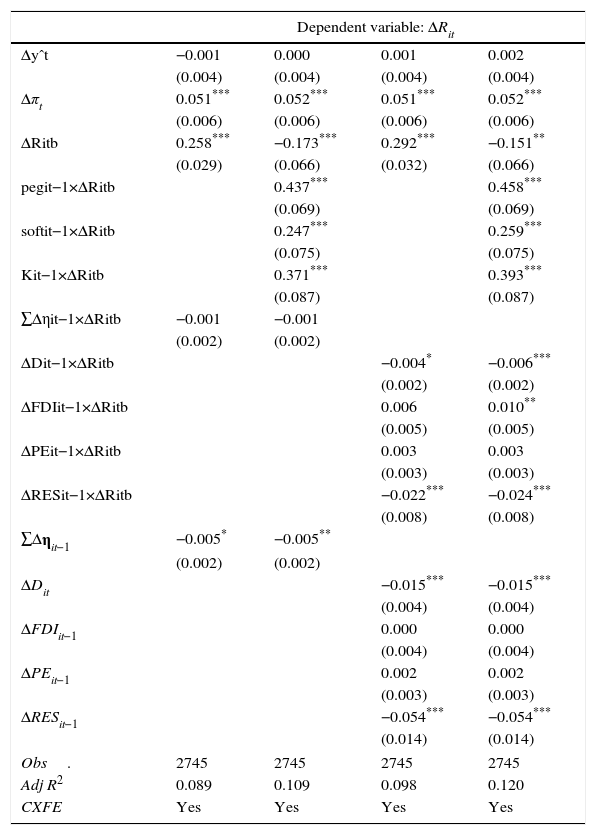
4.1.1

Longer sample period

The results presented earlier were drawn from a panel of 96 countries over the period 1992–2011. The limiting factor in the estimation was the data on the currency denomination of external debt, which is only available beginning in 1990 (and since the term in the regression is last period's change in net external assets, the earliest date to begin the regression is 1992). If we don’t need data on the currency denomination of external debt assets and liabilities, we can instead begin the estimation in 1973, like Klein and Shambaugh (2015).

The results for this longer sample period are presented in Table 3. We of course can’t fill in the last two columns of the earlier regression table, where we distinguish between domestic and foreign currency debt, but the results in the rest of the table are qualitatively identical. The change in net external debt liabilities and the change in central bank reserves are still the only two components of the change in the net external asset position that affect central bank autonomy. There is a quantitative change when using the longer sample period. The coefficients are smaller. This is due to the fact that this longer sample tends to place greater weight on the advanced economies in the sample, simply for data availability reasons. Advanced economies are less subject to surges and stops and the swings of the global financial cycle than many emerging markets, so advanced economy central banks are less inclined to sacrifice monetary policy autonomy and adopt a de facto exchange rate peg out of the fear of a stop in foreign financing of an external deficit.

Table 3.

Estimation results using a sample from 1973 to 2011.

	Dependent variable: ΔRit
Δyˆt	−0.001	0.000	0.001	0.002
	(0.004)	(0.004)	(0.004)	(0.004)
Δπt	0.051^***	0.052^***	0.051^***	0.052^***
	(0.006)	(0.006)	(0.006)	(0.006)
ΔRitb	0.258^***	−0.173^***	0.292^***	−0.151^**
	(0.029)	(0.066)	(0.032)	(0.066)
pegit−1×ΔRitb		0.437^***		0.458^***
		(0.069)		(0.069)
softit−1×ΔRitb		0.247^***		0.259^***
		(0.075)		(0.075)
Kit−1×ΔRitb		0.371^***		0.393^***
		(0.087)		(0.087)
∑Δηit−1×ΔRitb	−0.001	−0.001
	(0.002)	(0.002)
ΔDit−1×ΔRitb			−0.004^*	−0.006^***
			(0.002)	(0.002)
ΔFDIit−1×ΔRitb			0.006	0.010^**
			(0.005)	(0.005)
ΔPEit−1×ΔRitb			0.003	0.003
			(0.003)	(0.003)
ΔRESit−1×ΔRitb			−0.022^***	−0.024^***
			(0.008)	(0.008)
∑Δηit−1	−0.005^*	−0.005^**
	(0.002)	(0.002)
ΔDit			−0.015^***	−0.015^***
			(0.004)	(0.004)
ΔFDIit−1			0.000	0.000
			(0.004)	(0.004)
ΔPEit−1			0.002	0.002
			(0.003)	(0.003)
ΔRESit−1			−0.054^***	−0.054^***
			(0.014)	(0.014)
Obs .	2745	2745	2745	2745
Adj R^2	0.089	0.109	0.098	0.120
CXFE	Yes	Yes	Yes	Yes

Notes: Standard errors are in parenthesis.

*

Significance at the 10% level.

**

Significance at the 5% level.

***

Significance at the 1% level.

4.1.2

Correcting for valuation effects

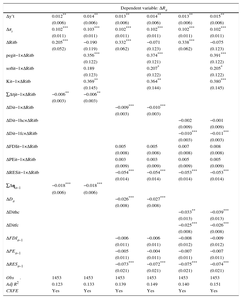
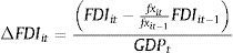
The terms in Δη_it are simply this year's stock of net external assets minus last year's stock of net external assets divided by GDP. These stocks are recorded in terms of U.S. dollars. Some variables, like reserves, are largely held in U.S. dollars, so it is fair to say that the flow of reserves in a given year is simply this year's USD stock minus last year's USD stock. However, as discussed by Bénétrix et al. (2015) when compiling data on the currency denomination of external assets and liabilities, it is fair to assume that portfolio equity and FDI are domestic currency denominated. Thus a depreciation in the exchange rate over the year would mean that there was a decrease in the USD value of external equity assets and liabilities, and thus subtracting last year's stock from this year's stock would make it seem as if there was a large decrease in equity assets and liabilities, even though there was no active accumulation of new assets or liabilities over the period.

A useful robustness test is to correct for these exchange rate valuation effects. After doing this, the terms in Δη_it are the changes to the net external asset position that are due to actual capital flows during the year, and not simply due to exchange rate changes, and the sum of the components of Δη_it is approximately equal to the current account (less net errors and omissions). These foreign exchange valuation changes will only affect a few components of Δη_it, domestic currency denominated debt, portfolio equity, and FDI. Earlier where the terms in Δη_it are simply this year's stock of net external assets minus last year's stock of net external assets divided by GDP:

When correcting for valuation effects, for these three components the entry in Δη_it is this year's stock of net external assets minus last year's stock multiplied by the gross change in the exchange rate over the year, all divided by GDP:

where fx_it is the end of the year value of the exchange rate (in terms of units of the domestic currency per USD).

The results from estimating the same regressions using these foreign exchange valuation corrected changes in net external assets are presented in Table 4. The table shows that there is very little qualitative or quantitative change in the results. The reason for this is simple. These foreign exchange valuation changes do not affect the two main components of the change in net external assets that were found to be significant, the change in foreign currency denominated debt and the change in reserves. These valuation changes affect the components that were found to be insignificant in these regressions, so there is almost no effect on the results from the estimation.

Table 4.

Regression results correcting for valuation effects in the change in net external assets.

	Dependent variable: ΔRit
Δyˆt	0.012^**	0.014^**	0.013^**	0.014^**	0.013^**	0.015^**
	(0.006)	(0.006)	(0.006)	(0.006)	(0.006)	(0.006)
Δπt	0.102^***	0.103^***	0.102^***	0.102^***	0.102^***	0.102^***
	(0.011)	(0.011)	(0.011)	(0.011)	(0.011)	(0.011)
ΔRitb	0.205^***	−0.190	0.332^***	−0.071	0.338^***	−0.075
	(0.052)	(0.119)	(0.062)	(0.123)	(0.062)	(0.123)
pegit−1×ΔRitb		0.356^***		0.374^***		0.391^***
		(0.122)		(0.121)		(0.122)
softit−1×ΔRitb		0.189		0.207^*		0.205^*
		(0.123)		(0.122)		(0.122)
Kit−1×ΔRitb		0.369^**		0.364^**		0.380^***
		(0.145)		(0.144)		(0.145)
∑Δηit−1×ΔRitb	−0.006^**	−0.006^**
	(0.003)	(0.003)
ΔDit−1×ΔRitb			−0.009^***	−0.010^***
			(0.003)	(0.003)
ΔDit−1hc×ΔRitb					−0.002	−0.001
					(0.009)	(0.009)
ΔDit−1fc×ΔRitb					−0.010^***	−0.011^***
					(0.003)	(0.003)
ΔFDIit−1×ΔRitb			0.005	0.005	0.007	0.008
			(0.008)	(0.008)	(0.008)	(0.008)
ΔPEit−1×ΔRitb			0.003	0.003	0.005	0.005
			(0.009)	(0.009)	(0.009)	(0.009)
ΔRESit−1×ΔRitb			−0.054^***	−0.054^***	−0.053^***	−0.053^***
			(0.014)	(0.014)	(0.014)	(0.014)
∑Δηit−1	−0.018^***	−0.018^***
	(0.006)	(0.006)
ΔDit			−0.026^***	−0.027^***
			(0.008)	(0.008)
ΔDithc					−0.033^**	−0.039^***
					(0.013)	(0.013)
ΔDitfc					−0.025^***	−0.026^***
					(0.008)	(0.008)
ΔFDIit−1			−0.006	−0.006	−0.008	−0.009
			(0.011)	(0.011)	(0.012)	(0.012)
ΔPEit−1			−0.005	−0.004	−0.007	−0.007
			(0.011)	(0.011)	(0.011)	(0.011)
ΔRESit−1			−0.073^***	−0.072^***	−0.075^***	−0.074^***
			(0.021)	(0.021)	(0.021)	(0.021)
Obs .	1453	1453	1453	1453	1453	1453
Adj R^2	0.123	0.133	0.139	0.149	0.140	0.151
CXFE	Yes	Yes	Yes	Yes	Yes	Yes

Notes: Standard errors are in parenthesis.

*

Significance at the 10% level.

**

Significance at the 5% level.

***

Significance at the 1% level.

4.1.3

A lagged interest rate in the monetary policy rule

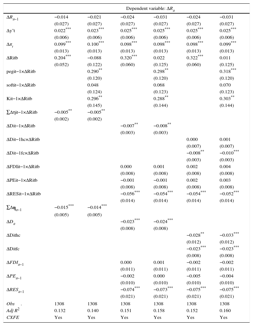
The estimation equation in (6) is derived from a Taylor rule where the only terms are inflation, the output gap, and exchange rate stability. Alternatively, one could consider the effect of including the lagged nominal interest rate in the monetary policy rule. In this case, the regression equation in (6) has one more right-hand side term: the lagged change in the home nominal interest rate, ΔR_it−1.

The results from these regressions are presented in Table 5. The table shows that the inclusion of the lagged interest rate in the Taylor rule has no effect on the estimates of the other coefficients. The change in net external debt liabilities and the change in central bank reserves are still the only two components of the change in the net external asset position that affect central bank autonomy.

Table 5.

Regression results where the lagged nominal interest rate is part of the estimated equation.

	Dependent variable: ΔRit
ΔRit−1	−0.014	−0.021	−0.024	−0.031	−0.024	−0.031
	(0.027)	(0.027)	(0.027)	(0.027)	(0.027)	(0.027)
Δyˆt	0.022^***	0.023^***	0.025^***	0.025^***	0.025^***	0.025^***
	(0.006)	(0.006)	(0.006)	(0.006)	(0.006)	(0.006)
Δπt	0.099^***	0.100^***	0.098^***	0.098^***	0.098^***	0.099^***
	(0.013)	(0.013)	(0.013)	(0.013)	(0.013)	(0.013)
ΔRitb	0.204^***	−0.088	0.320^***	0.022	0.322^***	0.011
	(0.052)	(0.122)	(0.060)	(0.125)	(0.060)	(0.125)
pegit−1×ΔRitb		0.290^**		0.298^**		0.318^***
		(0.120)		(0.120)		(0.120)
softit−1×ΔRitb		0.048		0.068		0.070
		(0.124)		(0.123)		(0.123)
Kit−1×ΔRitb		0.296^**		0.288^**		0.303^**
		(0.145)		(0.144)		(0.144)
∑Δηit−1×ΔRitb	−0.005^**	−0.005^**
	(0.002)	(0.002)
ΔDit−1×ΔRitb			−0.007^**	−0.008^**
			(0.003)	(0.003)
ΔDit−1hc×ΔRitb					0.000	0.001
					(0.007)	(0.007)
ΔDit−1fc×ΔRitb					−0.008^**	−0.010^***
					(0.003)	(0.003)
ΔFDIit−1×ΔRitb			0.000	0.001	0.002	0.004
			(0.008)	(0.008)	(0.008)	(0.008)
ΔPEit−1×ΔRitb			−0.001	−0.001	0.002	0.003
			(0.008)	(0.008)	(0.008)	(0.008)
ΔRESit−1×ΔRitb			−0.056^***	−0.054^***	−0.054^***	−0.052^***
			(0.014)	(0.014)	(0.014)	(0.014)
∑Δηit−1	−0.015^***	−0.014^***
	(0.005)	(0.005)
ΔDit			−0.023^***	−0.024^***
			(0.008)	(0.008)
ΔDithc					−0.028^**	−0.033^***
					(0.012)	(0.012)
ΔDitfc					−0.023^***	−0.023^***
					(0.008)	(0.008)
ΔFDIit−1			0.000	0.001	−0.002	−0.002
			(0.011)	(0.011)	(0.011)	(0.011)
ΔPEit−1			−0.002	0.000	−0.005	−0.004
			(0.010)	(0.010)	(0.010)	(0.010)
ΔRESit−1			−0.074^***	−0.073^***	−0.075^***	−0.075^***
			(0.021)	(0.021)	(0.021)	(0.021)
Obs .	1308	1308	1308	1308	1308	1308
Adj R^2	0.132	0.140	0.151	0.158	0.152	0.160
CXFE	Yes	Yes	Yes	Yes	Yes	Yes

Notes: Standard errors are in parenthesis.

**

Significance at the 5% level.

***

Significance at the 1% level.

4.1.4

Post-inflation targeting subsample

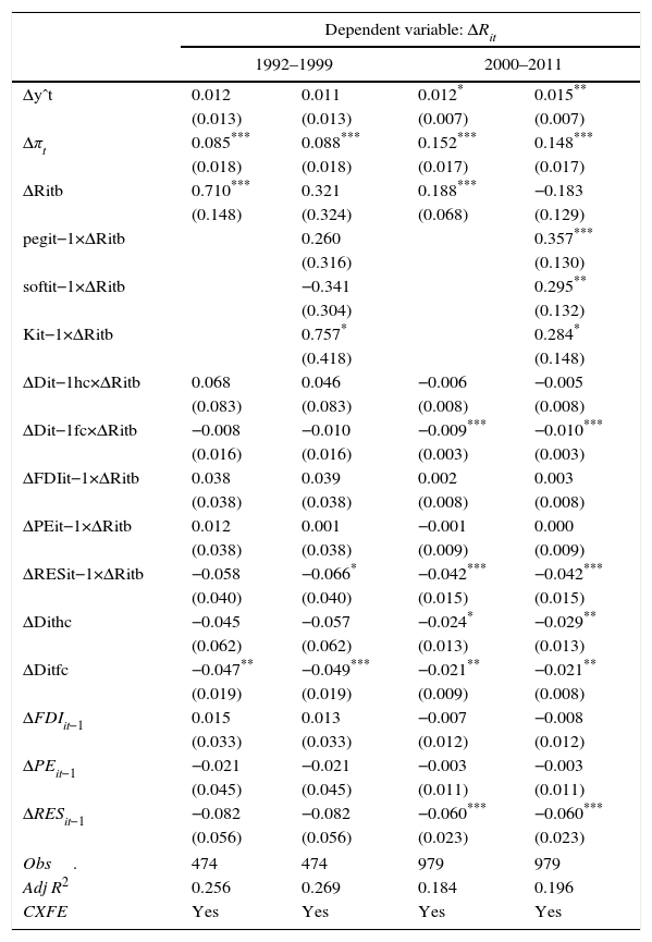
The main sample period in this study is 1992–2011. Inflation targeting was first adopted by the Reserve Bank of New Zealand in 1989, and by the beginning of the sample inflation targeting had spread to a few other (mostly) developed countries like Canada and Sweden. But the real wave of adoption of inflation targeting by both developed and developing countries came around the turn of the century. It is thus natural to ask whether these regression results are simply the feature of an earlier, pre-IT, monetary policy?

To test this claim, we split the sample into two periods, the first from 1992 to 1999 and the second from 2000 to 2011, and recalculate the benchmark regression results in each subsample. This is presented in Table 6. The first and most obvious thing to notice is that between these two subperiods, there is a large increase in the estimated coefficient on inflation and a fall in the estimated coefficient on the foreign interest rate. This is a sign that between the 1990's and 2000's subperiods, many countries in the sample changed their monetary policy from exchange rate targeting to inflation targeting. In fact the results show that during the earlier subsample, a country with an open capital account would adjust their policy rate nearly one-for-one with changes in the base country interest rate, a sign of exchange rate targeting.

Table 6.

Regression results in pre- and post-1999 subsamples.

	Dependent variable: ΔRit
	1992–1999		2000–2011
Δyˆt	0.012	0.011	0.012^*	0.015^**
	(0.013)	(0.013)	(0.007)	(0.007)
Δπt	0.085^***	0.088^***	0.152^***	0.148^***
	(0.018)	(0.018)	(0.017)	(0.017)
ΔRitb	0.710^***	0.321	0.188^***	−0.183
	(0.148)	(0.324)	(0.068)	(0.129)
pegit−1×ΔRitb		0.260		0.357^***
		(0.316)		(0.130)
softit−1×ΔRitb		−0.341		0.295^**
		(0.304)		(0.132)
Kit−1×ΔRitb		0.757^*		0.284^*
		(0.418)		(0.148)
ΔDit−1hc×ΔRitb	0.068	0.046	−0.006	−0.005
	(0.083)	(0.083)	(0.008)	(0.008)
ΔDit−1fc×ΔRitb	−0.008	−0.010	−0.009^***	−0.010^***
	(0.016)	(0.016)	(0.003)	(0.003)
ΔFDIit−1×ΔRitb	0.038	0.039	0.002	0.003
	(0.038)	(0.038)	(0.008)	(0.008)
ΔPEit−1×ΔRitb	0.012	0.001	−0.001	0.000
	(0.038)	(0.038)	(0.009)	(0.009)
ΔRESit−1×ΔRitb	−0.058	−0.066^*	−0.042^***	−0.042^***
	(0.040)	(0.040)	(0.015)	(0.015)
ΔDithc	−0.045	−0.057	−0.024^*	−0.029^**
	(0.062)	(0.062)	(0.013)	(0.013)
ΔDitfc	−0.047^**	−0.049^***	−0.021^**	−0.021^**
	(0.019)	(0.019)	(0.009)	(0.008)
ΔFDIit−1	0.015	0.013	−0.007	−0.008
	(0.033)	(0.033)	(0.012)	(0.012)
ΔPEit−1	−0.021	−0.021	−0.003	−0.003
	(0.045)	(0.045)	(0.011)	(0.011)
ΔRESit−1	−0.082	−0.082	−0.060^***	−0.060^***
	(0.056)	(0.056)	(0.023)	(0.023)
Obs .	474	474	979	979
Adj R^2	0.256	0.269	0.184	0.196
CXFE	Yes	Yes	Yes	Yes

Notes: Standard errors are in parenthesis.

*

Significance at the 10% level.

**

Significance at the 5% level.

***

Significance at the 1% level.

The coefficients on the interaction between the foreign interest rate and central bank reserves or the stock of foreign currency denominated debt are significant in the later subsample, indicating that the main conclusion of this paper, that a deterioration in the net foreign asset position leads the central bank to place more weight on movements in the foreign interest rate, continues to hold in the post-IT subsample. The point estimates of these coefficients are about the same in both subsamples, but they are not significant in the earlier subsample due to high standard errors. But these results from different subsamples suggest that the channel where the loss of central bank reserves or the accumulation of foreign currency debt leads a central bank to sacrifice monetary policy autonomy is not simply a feature of an exchange rate targeting stance of monetary policy and continues to hold in countries that have adopted inflation targeting.

5

Conclusion

Mechanically, a central bank with a floating currency has complete monetary policy autonomy and can do whatever they want with their interest rate instrument. But when setting policy, central banks face trade-offs. One of these trade-offs is between the need to stabilize the domestic economy and the need to stabilize capital flows, the exchange rate, and the external accounts.

A country's economic fundamentals can affect this trade-off. A country with a current account surplus that is accumulating central bank reserves and claims on the rest of the world has little to fear from a sudden stop in capital inflows.⁸ Thus the central bank in this country can focus on the domestic economy and has no need to trade-off domestic stabilization for exchange rate and capital flow stabilization. On the other hand a country with a current account deficit, especially a deficit financed by reserve depletion or the accumulation of foreign currency denominated debt, has a lot to fear from a sudden stop in capital inflows, and the central bank will be forced to use their interest rate to attract capital inflows and thus stabilize the external accounts, even if that comes at the cost of destabilizing the domestic economy.

Nowhere is this more evident than when a central bank drastically raises interest rates in an attempt to curtail a sudden drop in net capital inflows. The central bank of Russia's increase of 750 basis points in December 2014 or the central bank of Turkey's increase of 550 basis points in January 2014 are just two recent examples.

But apart from these dramatic cases, this paper shows that even modest reserve depletion or modest increases in foreign currency denominated debt can lead a central bank with a floating currency to adopt a de facto exchange rate peg. The estimates in this paper show that reserve depletion of 7% of GDP over the past year can so change the trade-offs faced by the central bank that they would be willing to abandon the floating currency and adopt a de facto peg in the interest of stabilizing capital flows.

This in turn has implications for the global effect of a monetary tightening by a base country central bank like the Federal Reserve. Since many central banks that are concerned about the stability of capital flows and their external account would be tempted to mimic Fed action in raising interest rates, the actual effect of Fed tightening on global liquidity is greater than it would have been if the Fed acted alone.

Conflict of interests

The author declares that he has no conflict of interest.