

This paper characterizes analytically the adjustment of an open economy with a stock collateral constraint to fundamental and nonfundamental shocks. In the model, external borrowing is limited by the value of physical capital. Three results are established: (1) Adjustment to external shocks is nonlinear. In response to small negative output shocks, the economy adjusts as prescribed by the intertemporal approach to the current account, with increases in debt, deficits in the trade and current account balances, and no significant movement in the price of collateral. By contrast, in response to large negative output shocks the economy experiences a sudden stop with debt deleveraging, trade and current account reversals, and a Fisherian deflation of asset prices. (2) Generically, weak fundamentals (low output and high external debt) give rise to multiple equilibria. (3) In this case, the economy is prone to self-fulfilling sudden stops driven by downward revisions of expectations about the value of collateral.
Este artículo caracteriza de manera analítica el ajuste de una economía abierta con restricciones sobre el colateral a choques fundamentales y no fundamentales. En el modelo, el endeudamiento externo está limitado por el valor del capital físico. Se establecen tres resultados: (1) El ajuste a los choques externos es no lineal. En respuesta a choques de producción negativos pequeños, la economía se ajusta según lo dictado por el enfoque intertemporal de la cuenta corriente, con incrementos en la deuda, los déficits en la balanza comercial y de cuenta corriente, y sin movimientos significativos en el precio del colateral. Al contrario, en respuesta a los choques de producción negativos grandes la economía experimenta una parada súbita en los flujos de capitales con reducción del apalancamiento de la deuda, reversión de la balanza comercial y de cuenta corriente, y una deflación de Fisher de los precios de los activos. (2) En líneas generales, unos fundamentales débiles (baja producción y deuda externa alta) dan lugar a equilibrios múltiples. (3) En este caso, la economía es susceptible de paradas súbitas autocumplidas impulsadas por las revisiones a la baja de las expectativas acerca del valor del colateral.
This paper characterizes analytically the adjustment of an open economy with a stock collateral constraint to small and large fundamental shocks and to nonfundamental (or sunspot) shocks. In a model driven by productivity shocks, we derive a threshold for the magnitude of negative shocks. For negative realizations of the shocks that are smaller than this threshold, the presence of the collateral constraint does not affect the adjustment. In particular, in response to a negative productivity shock, the economy adjusts as prescribed by the intertemporal approach to the current account. That is, it borrows internationally to smooth consumption, which causes a deterioration of the trade balance and a deterioration of the current account. Along this adjustment, the equilibrium price of collateral is unaffected. By contrast, if the size of the negative productivity shock is larger than the aforementioned threshold, then the presence of the constraint amplifies the adjustment. Instead of borrowing from abroad to smooth consumption, the economy is forced to deleverage. As a consequence the current account and the trade balance display surpluses, and consumption contracts by more than the decline in output. In addition, the deleveraging induces a massive desire to sell capital, resulting in a Fisherian deflation of Tobin's q and fire sales.
These results complement existing ones derived numerically in the context of calibrated models. For example, in a model calibrated to Mexico Mendoza (2010) finds that the unconditional standard deviation of output is about the same in versions of his model with and without the stock collateral constraint—a finding he interprets as indicating that the presence of collateral constraints does not amplify regular business cycles. At the same time, Mendoza finds that aggregate dynamics are amplified in periods in which negative shocks are so large that the collateral constraint binds.
Open economies with collateral constraints are vulnerable not just to fundamental sources of uncertainty, but also to nonfundamental ones. A problem that plagues this type of economies is that under plausible parameterizations, the equilibrium may fail to be unique. The possibility of equilibrium multiplicity in open-economy models with collateral constraints has been suggested by Mendoza (2005) and by Jeanne and Korinek (2010). The former study considers a model with a flow collateral constraint in which external borrowing is limited by the value of output and the latter considers a model with a stock collateral constraint, like the one studied in the present analysis. Both papers present a heuristic analysis of the problem and are focused on providing conditions for uniqueness. In this regard, the contribution of the present paper is to prove the existence of multiple equilibria formally and to characterize the associated equilibrium dynamics.
Essentially, the problem that arises is that if an unconstrained equilibrium exists, often a second equilibrium exists in which the collateral constraint is binding. This situation is more likely to occur when economic fundamentals are weak, that is, when the country is highly indebted and output is depressed. In the equilibrium with the binding collateral constraint, negative beliefs bring the price of capital down, causing a tightening of the collateral constraint. In turn, the decline in the value of collateral forces agents to deleverage leading to a fire sale of capital. Because the stock of capital is fixed in the short run, the fire sale depresses asset prices, validating the negative beliefs. The resulting self-fulfilling crisis carries all the characteristics of a sudden stop, namely, reversals in the trade and current-account balances and a contraction in aggregate demand. In addition, we show that these confidence crises are welfare decreasing, as they force households to deviate from consumption smoothing. In this sense, the deleveraging that occurs in a self-fulfilling crisis can be interpreted as underborrowing.
The remainder of the paper is organized in six sections. Section 2 presents an open economy model with a stock collateral constraint. Section 3 characterizes the steady-state equilibrium. Section 4 characterizes the equilibrium adjustment to regular-sized shocks. Section 5 characterizes the equilibrium adjustment to large shocks. Section 6 proves the existence of multiple equilibria and characterizes the dynamics of self-fulfilling financial crises. Section 7 concludes.
2The modelConsider a perfect-foresight small open economy populated by a large number of households with preferences given by the utility function
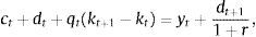
where ct denotes consumption and β∈(0, 1) denotes the subjective discount factor. The sequential budget constraint of the household is assumed to be of the formwhere dt denotes debt acquired in period t−1 and due in period t, kt denotes the stock of physical capital in period t, qt denotes the price of one unit of capital in terms of consumption in period t, yt denotes output in period t, and r>0 denotes a constant interest rate on debt. For simplicity, we assume a zero depreciation rate of physical capital. Output is produced with the technologywhere At is an exogenous and deterministic productivity factor, and α∈(0, 1) is a parameter.

Assume that borrowing is limited by a constant fraction κ>0 of the value of physical capital. Formally,
The parameter κ can be interpreted as the fraction of assets that lenders could seize from the borrower in the event of a default. Under this interpretation, the above borrowing constraint is an incentive compatibility restriction, which ensures that the borrower never walks away from his external debt obligations.1
The above collateral constraint pertains to the class of stock collateral constraints, because the pledgeable object, physical capital, is a stock. Because the price of capital, qt, is taken as given by the individual household, but is endogenously determined in equilibrium, the collateral constraint introduces a pecuniary externality. An increase in the aggregate demand for capital drives up qt, allowing the individual household to borrow more. Similarly, a fall in the aggregate demand for capital drives qt down, which may force households to deleverage. Individual households understand this mechanism, but fail to internalize it, because, due to their atomistic nature they correctly realize that their own demand for capital is too small to affect its price. This externality and its implications for prudential policy was first stressed in the context of an open economy model by Auernheimer and García-Saltos (2000). It has been extensively studied by subsequent authors in the context of both stock and flow collateral constraint models.2
The household chooses sequences ct>0, dt+1, and kt+1≥0 to maximize its lifetime utility subject to the sequential budget constraint (1), the production technology (2), and the collateral constraint (3), taking as given the sequence of prices qt and the initial conditions d0 and k0. The Lagrangian associated with this optimization problem is
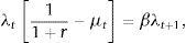
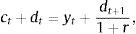
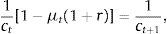
where βtλt and βtλtμt are the Lagrange multipliers associated with the sequential budget constraint and the collateral constraint, respectively. The associated first-order conditions with respect to ct, dt+1, and kt+1 are, respectively,andOptimality condition (5) equates the marginal costs and benefits of increasing dt+1. The marginal benefit is 1/(1+r) units of consumption in t, which is equivalent to λt/(1+r) units of utility. In normal times, i.e., when the collateral constraint is not binding, the marginal cost of increasing dt+1 by one unit is the sacrifice of one unit of consumption in t+1, which is equivalent to βλt+1 units of utility. When the collateral constraint is binding, the marginal cost of an additional unit of debt increases by μt units of goods or λtμt units of utility, reflecting a shadow punishment for trying to increase debt when the household is up against the limit. Similarly, optimality condition (6) equates the marginal cost and benefit of purchasing an additional unit of capital. The marginal cost of capital is its price, qt. During normal times, the marginal benefit of an additional unit of capital purchased in t is the additional output it generates in t+1, or the marginal product of capital αAt+1kt+1α−1, plus the price at which this additional unit of capital can be sold in period t+1, qt+1. When the collateral constraint binds, the benefit of an additional unit of capital increases by κμtqt, reflecting its contribution to relaxing the borrowing constraint.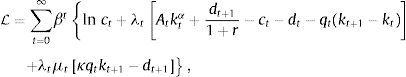


The optimality conditions associated with the household's optimization problem also include the Kuhn-Tucker non-negativity and slackness conditions
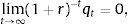
andBecause preferences display no satiation, the optimality conditions include the terminal condition3

To facilitate the characterization of equilibrium, assume that the aggregate supply of capital is fixed and equal to k>0. Therefore, in equilibrium we have
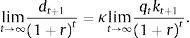
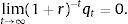
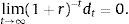
for all t. The price of capital must be nonnegative, that is, qt≥0. In addition, we restrict attention to equilibria in which the price of capital does not display a bubble, that is, equilibria in which qt grows at a rate strictly less than r. Formally, we imposeConditions (9)–(11) imply that the present discounted value of debt must converge to zero, that is,In turn, this condition together with the sequential budget constraint (1) and the market clearing condition (10) implies d0=∑t=0∞yt−ct(1+r)t, which states that the present discounted value of future expected trade balances must cover the country's initial net external debt position. Finally, we assume that the subjective and market discount factors are equal,

A (bubble-free) competitive equilibrium is then a set of sequences ct>0, dt+1, μt≥0, and qt≥0 satisfying
given d0 and the exogenous sequences At and yt≡Atkα. Eq. (15) together with the requirement that ct>0 implies that μt<1/(1+r)<1.3The steady-state equilibrium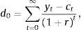

Suppose that the productivity factor At is constant over time and equal to A for all t≥0, where A is a positive parameter. Then the path of output is also constant and equal to yt=y≡Akα. In this section we show that under these conditions, there exists a steady-state equilibrium, that is, an equilibrium in which all variables are constant over time.
A steady-state equilibrium is a set of constant sequences ct=c*>0, dt+1=d*, μt=μ*≥0, and qt=q*≥0 that satisfy equilibrium conditions (13)–(19) given d0. What does the steady state look like? Because consumption is constant over time, Eq. (15) implies that μ*=0. This means that in the steady state the economy is not borrowing constrained. Then, Eq. (16) becomes qt=βqt+1+βαy/k. Since β∈(0, 1), the unique stationary solution to this expression is
which intuitively says that the steady-state price of capital equals the present discounted value of current and future marginal products of capital.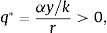
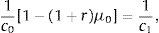
Evaluating the sequential budget constraint (14) in any period t>0 implies that the steady-state level of consumption is given by
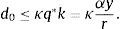
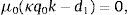
This is a familiar characteristic of open economy models in the steady state. It says that households consume their permanent income, given by the sum of nonfinancial income, y, and interest income, −rd*/(1+r). Using the above expression to eliminate c0 from the sequential budget constraint in period 0 yieldsThus, the steady-state level of debt depends on (is actually equal to) the level of debt inherited from the past in period 0. Because the net debt position is constant in the steady state, we have that the steady-state current account, denoted ca*, is nil,The steady-state trade balance, tb*≡y−c*, equals the interest obligations on external debt,Finally, it is natural to ask what levels of debt are sustainable in the steady state. Taken together, the above expression for steady-state consumption and the requirement that consumption be positive impose the following upper bound on external debtwhich is a natural debt limit, above which servicing the debt would cause households to starve. The collateral constraint introduces a second upper bound on debt, given byComparing the debt bounds (21) and (22) we have that as long as κ<1, the latter will be the more restrictive bound. Throughout the paper, we assume, as in much of the related literature, thatThis restriction says that leverage cannot exceed one hundred percent. It then follows that the maximum value of debt sustainable in the steady state is given by condition (22). Any level of debt satisfying this condition can be supported as a steady-state equilibrium.4Frictionless adjustment to regular shocks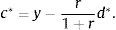


An important theme of the collateral-constraint literature is that this type of financial friction affects the adjustment of economies to large, unusual shocks, but not to regular-sized shocks. We illustrate this principle by characterizing the equilibrium dynamics implied by the present model in response to regular and large negative productivity shocks. The analysis will make clear what constitutes a regular and a large shock in the present environment.
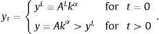
Suppose that the economy was in a steady state until period −1. Suppose also that in period 0 the productivity factor At unexpectedly falls from A to AL<A, and returns to A permanently starting in period 1. This sequence of productivity shocks gives rise to the following path for output
The question we wish to answer here is under what conditions the adjustment to the negative productivity shock will be frictionless. By a frictionless adjustment we mean one that would occur if the collateral constraint was not in place. The equilibrium conditions of the frictionless economy are (13)–(16) and (19), with μt=0 for all t.
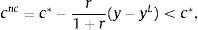
Let ctnc denote the equilibrium level of consumption in period t in the economy without the collateral constraint (nc for no collateral constraint). Then, Eq. (15) implies that
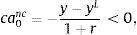
for all t≥0, where cnc is a constant. So equilibrium consumption is perfectly smooth in the economy without the collateral constraint. This is a consequence of the assumption that β(1+r)=1. Evaluating the intertemporal resource constraint (13) at ct=cnc for all t≥0 implies that cnc is given byfor all t≥0, where, as before, c*=y−r/(1+r)d0 denotes the level of consumption that would have occurred in the absence of the negative productivity shock in period 0. Now using the sequential resource constraint (14), we obtain a constant equilibrium path of external debt given byfor all t≥1. In period 0, both the current account and the trade balance deteriorate,andBecause the productivity shock is temporary, the household borrows an amount close to the output shock (y−yL) to smooth consumption. More precisely, the household borrows (y−yL)/(1+r). This increases debt in period 1 by exactly y−yL. The household finds it optimal to pay the interest on the additional debt every period, but not the principal, so consumption falls slightly by the increased interest service, r(y−yL)/(1+r).

Finally, because, by definition, in the economy without the collateral constraint μt=0, Eq. (16) implies that the price of capital is unchanged by the productivity shock,
for all t.
Under what conditions does the equilibrium in the economy without the collateral constraint coincide with the equilibrium in the economy with the collateral constraint? For this to be the case, it is necessary that the collateral constraint (18) be satisfied when evaluated at dnc and qnc, that is, it is necessary that
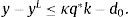
Using the solution for dnc obtained above yields the conditionThe right-hand side of this expression is the slack in the collateral constraint prior to period 0. The left-hand side is the output contraction in period 0. Thus, an output contraction in period 0 induces a frictionless adjustment if it is smaller than the slack in the collateral constraint prior to the shock. It follows that the adjustment to an output contraction is more likely to be frictionless the smaller is the contraction itself, the smaller is the level of debt prior to the contraction, d0, and the less severe is the financial friction, i.e., the larger is κ. In the context of this model, we will refer to contractions that satisfy (23) as regular-sized contractions.5Adjustment to large shocks
Continue to assume that the economy was in a steady state until period −1. But now assume that the contraction of output in period 0, y−yL, is so large that condition (23) is not satisfied, so that
In the context of the present model, we define a large contraction as one that satisfies the above inequality.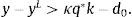
What does the equilibrium look like when the economy is hit by a large negative shock? We wish to show that a large negative output shock causes a Fisherian deflation, that is, a fall in the price of capital, qt, and deleveraging, that is, a reduction in net external debt, dt. The first thing to note is that the collateral constraint must bind in at least one period, that is, μt must be strictly positive and condition (3) must hold with equality for some t≥0. To see this, suppose, on the contrary that μt=0 for all t. Then, by the debt Euler equation (15), ct is constant over time, which implies, by the intertemporal resource constraint (13), that ct=cnc. The sequential budget constraint (14) then yields dt+1=dnc, and the capital Euler equation (16) yields qt=q* for all t≥0. But, by condition (24), this allocation violates the collateral constraint in period 0. This establishes that in response to a large negative output shock μt must be positive in at least one period.
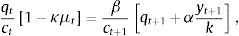
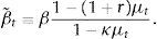
Consider now the equilibrium value of capital, qt, in the period in which μt is strictly positive. To this end, rewrite the capital Euler equation (16) as
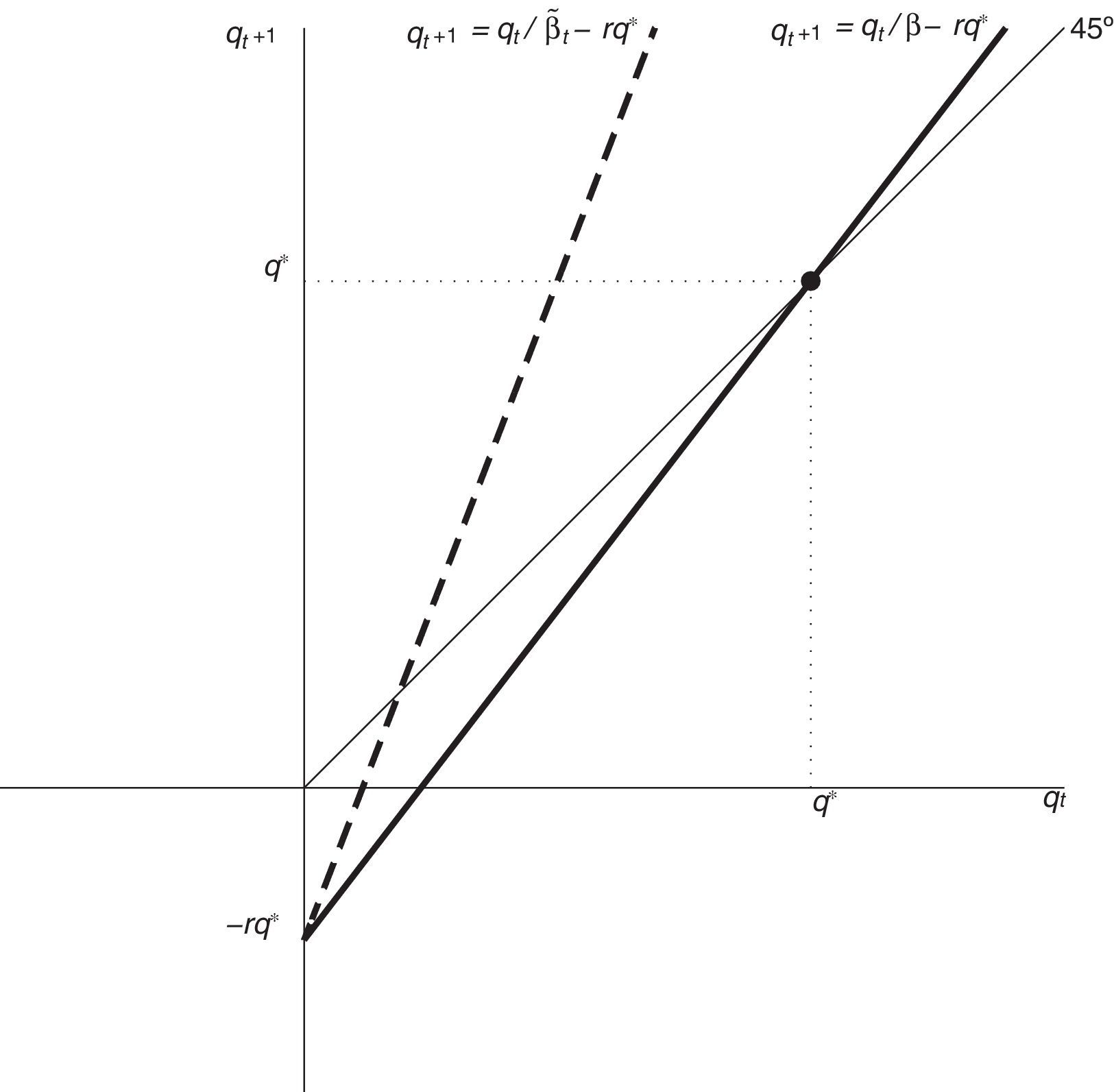
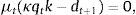
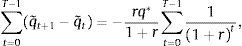
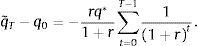
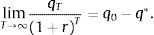
where β˜t is given byNote that 0<β˜t≤β, that β˜t=β when μt=0, and that β˜t<β when μt>0 (recall that we are assuming that κ<1 and that r>0). According to this expression, in determining their demand for assets (in this case physical capital), households behave as if they became more impatient in periods in which the collateral constraint binds. Fig. 1 displays the phase diagram of the price of capital in the space (qt, qt+1). The heavy solid line corresponds to the case β˜t=β, and the broken line to the case β˜t<β. When β˜t=β, the stationary state of qt is given by q*. It is clear from the phase diagram that, regardless of the value of β˜t, a value of qt larger than q* would trigger an explosive path. In principle, a growing path of qt could be consistent with equilibrium if it does not violate the no-bubble constraint (19). It turns out, however, that this constraint is violated for any initial condition q0>q*. To see this, note that since 1/β˜t≥1+r, it suffices to show that any path of qt with initial condition q0>q* violates the no-bubble constraint for β˜t=β. Now evaluate (25) at β˜t=β, divide both sides by (1+r)t+1, and sum for T−1 periods to getwhere q˜t≡qt/(1+r)t is the present discounted value of the price of capital. This object must converge to zero in order for the no-bubble constraint to be satisfied. We can write the above expression asLetting T→∞ in the above expression, we obtainIt follows that the no-bubble constraint is violated for any initial condition q0>q*. As we will see shortly, however, q0<q* does not necessarily lead to a violation of the no-bubble constraint or of the nonnegativity constraint on qt, because in that case, changes in β˜t can prevent qt from imploding.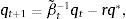

So far, we have established that in equilibrium qt≤q*, for all t≥0 and that a large negative output shock in period 0 causes the collateral constraint to bind in at least one period. It remains to show that when the collateral constraint binds, qt and dt+1 fall.
Let T≥0 denote the first period in which μt is strictly positive. This means that β˜T−1>β−1>1. It then follows from Eq. (25), that if qT were to equal q*, then qT+1 would be strictly greater than q*, which, by the arguments given above, would be inconsistent with equilibrium. It follows that qT must be strictly less than q*. From periods 0 to T−1, β˜t=β. Therefore, in period T−1, Eq. hyperlinkeq:ovb_q_q_betatilde((25)) becomes
which says that qT−1 is a weighted average of qT and q*. Since qT<q*, it follows that qT−1<q*. By induction we have thatThis establishes an important prediction of the present model, namely, that a large contraction in output is necessarily accompanied by a Fisherian deflation.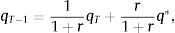

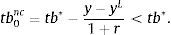
Furthermore, both debt and consumption fall in period 0 relative to the values they would have taken in the absence of the collateral constraint. To see this, note that the debt Euler equation (15) and the fact that μt≥0 for all t, imply that in any equilibrium consumption is nondecreasing from period 0 on. The debt Euler equation and the fact that μT>0, also imply that consumption must increase in period T+1, that is, cT+1>cT. Since μt=0 for all t<T, we have, again by the debt Euler equation, that consumption is constant over this period, ct=cT for t≤T. Now, by the intertemporal resource constraint (13), the present discounted value of consumption must be the same in the economy with the collateral constraint and in the economy without that constraint. So we have two paths of consumption with the same present discounted value, one of which is flat (the one associated with the economy without the collateral constraint) and the other is nondecreasing and strictly increasing in at least one period (the one associated with the economy with the collateral constraint). It must therefore be the case that the initial value of the latter consumption path is strictly lower than the initial value of the former path. That is, c0 must be strictly smaller than c0nc. The sequential budget constraint (14) evaluated at t=0 then directly implies that d1 must be strictly less than d1nc. This establishes that a large negative output shock in period 0 causes deleveraging in that period. It also follows that the economy with a collateral constraint experiences smaller deteriorations of the trade balance and current account relative to the economy without the collateral constraint, ca0>ca0nc and tb0>tb0nc.
In summary, we have shown that the presence of a collateral constraint causes a Fisherian deflation, debt deleveraging, and an amplification of the contraction in aggregate demand in response to a large negative output shock. The intuition behind this central result is as follows. In response to a temporary negative output shock, households would like to borrow in order to smooth consumption. If the shock is large enough, the desired level of debt will exceed the borrowing limit κq*k. From an individual point of view, the household has an incentive to sell capital, because, one unit of capital sells for q* units of consumption goods. However, the household cannot increase consumption by quite this amount, because reducing capital by one unit tightens the collateral constraint by κq* units, so the household must use this amount to reduce debt, leaving (1−κ)q* units for additional consumption. Now, every household wants to sell capital. This situation is known as a fire sale. But this is impossible in equilibrium because the stock of capital is fixed. For the capital market to clear, the price of capital, qt, must fall, that is, a Fisherian debt deflation must occur. If the collateral constraint was binding or close to binding before the shock (i.e., d0 close to κq*k), then the fall in q0 would force households to reduce their net debt positions, d1<d0, that is to say, it would force households to deleverage. This is exactly the opposite of what happens in the absence of a collateral constraint. In that case, a large negative output shock induces an increase in household indebtedness.
Once the output shock is over (period 1), the economy can reach an equilibrium in which qt returns to its steady-state value q* and debt is forever equal to d1. To see that this is the case, notice that in such an equilibrium the collateral constraint would not bind after period 0, because dt=d1=κq0k<κq*k, for all t≥1. This means that μt=0, for t≥1, which by the Euler equation (15) implies that consumption is also constant. Notice that the country emerges from the financial crisis stronger than it entered, because, after period 0, consumption is permanently higher, debt is permanently lower, and the collateral constraint may be more relaxed. However, this strength comes at a cost, because the fall in consumption in period 0 reduces lifetime welfare.
6Self-fulfilling financial crisesThus far, we have focused attention on the aggregate effects of fundamental shocks. In this section, we study the vulnerability of open economies with collateral constraints to nonfundamental (or sunspot) shocks. A key result of this section is the demonstration that generally weak economic fundamentals give rise to multiple equilibria. We then characterize the dynamics triggered by self-fulfilling financial crises.
To isolate the role of nonfundamental shocks, we eliminate fundamental sources of aggregate fluctuations by assuming that productivity is constant over time. Thus, we set yt=y for all t≥0, where y>0 is a constant. Suppose also that
where q* is the steady-state price of capital given in equation (20). This restriction guarantees that the initial level of debt does not violate the collateral constraint when q0=q*. Then, the analysis presented in Section 3 implies that there exists an equilibrium in which the economy is at a steady state starting in period 0. In this equilibrium, ct=c*≡y−d0r/(1+r)>0, dt=d0, qt=q*, and μt=0 for all t≥0. Along this equilibrium path, the collateral constraint never binds. We therefore refer to this equilibrium as the unconstrained equilibrium. We wish to show that in general there exists a second equilibrium in which the collateral constraint binds in period 0. In this second equilibrium, the economy suffers a Fisherian deflation and debt deleveraging in the initial period. In addition, the real allocation is welfare inferior to the one associated with the unconstrained equilibrium. We refer to this second equilibrium as the constrained equilibrium.
In the constrained equilibrium we consider here, the economy reaches a steady state in period 1. To see that a steady state equilibrium starting in period 1 exists, recall from Section 3, that the only requirement for the existence of a steady-state equilibrium starting in period 1 is that the collateral constraint be satisfied. This is indeed the case because dt+1=d1=κq0k≤κq*k=κqtk for all t≥1. The first equality follows from the assumption that the economy is in a steady state starting in period 1, the second follows from our assumption that the collateral constraint is binding in period 0, the weak inequality follows from the upper bound qt≤q* derived earlier, and the last equality from the fact that in a steady-state equilibrium qt=q* for all t.
Taking into account that the economy reaches a steady state in period 1, the complete set of equilibrium conditions, Eqs. (13)–(19), collapses to the following system of five equations in the five unknowns, c0>0, c1>0, d1, q0≥0, and μ0≥0,
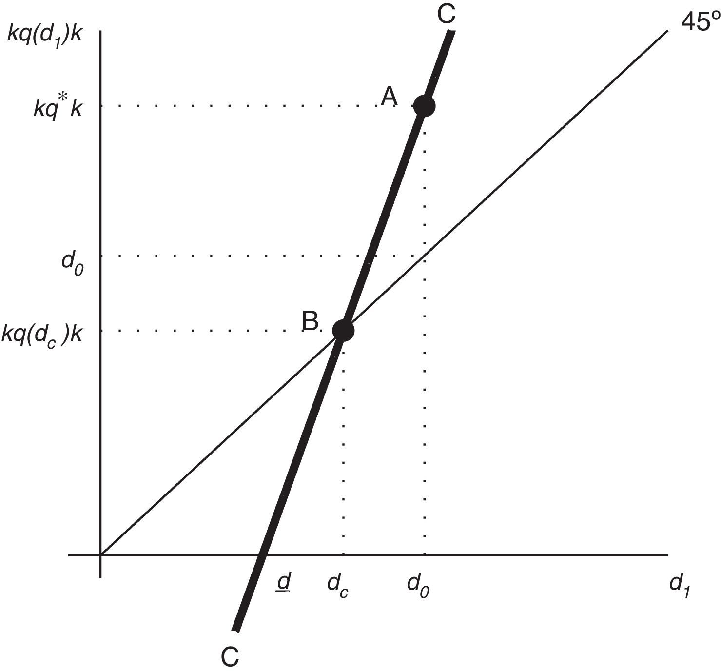
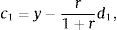
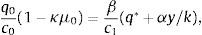
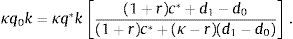
Now solve (27)–(30) for q0 as a function of d1 to obtainFig. 2 displays with a thick solid line the graph of κq0k as a function of d1 implied by this equation. The locus CC¯ is the collection of pairs (d1, κq0k) that guarantee that equilibrium conditions (27)–(30) are satisfied. Recalling that 1+r>1>κ, it can readily be shown that CC¯ is upward sloping. Also, CC¯ crosses the point (d0, κq*k), which is labeled A in the figure. Note that point A lies above the 45° line, reflecting the assumption that d0≤κq*k. We have already shown that d1=d0 represents a steady state equilibrium. To see that there may exist a second equilibrium, begin by noting that all points of CC¯ that lie on or above the 45° line satisfy the collateral constraint (32). Consider now the value of d1 at which the locus CC¯ crosses the horizontal axes. This value of d1 is denoted d_ in the figure. Suppose that, as shown in the figure, d_ is positive. (We will discuss shortly conditions for this to be the case.) Then, CC¯ must necessarily cross the 45° line at some level of debt in the open interval (d_,d0). This value of d1 is denoted dc and the intersection point is marked with the letter B in the figure. Because B is on CC¯ and on the 45° line, it satisfies equilibrium conditions (27)–(30) and the collateral constraint (32). Moreover, at B the collateral constraint holds with equality, which means that the slackness condition (31) is satisfied. To establish that point B represents an equilibrium, it remains to show that d1=dc implies c0>0, c1>0 and μ0≥0. To this end, note that the numerator of the expression within brackets in Eq. (33) is (1+r)c0. At d1=d_, the numerator is nil, so (1+r)c0=0. At d1=d0, (1+r)c0=(1+r)c*. Since by (27) and (28), c0 is increasing in d1, it follows that at d1=dc, (1+r)c0 must be strictly positive and less than (1+r)c*. It follows that d1=dc implies 0<c0<c*. Also, the fact that dc<d0 implies, by the sequential resource constraint (28), that c1>c*. So we have that d1=dc implies 0<c0<c*<c1. The debt Euler equation (29) then implies that μ0 is positive.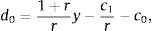


This establishes the existence of a second equilibrium in which q0<q* and d1<d0, that is, an equilibrium with a Fisherian deflation and debt deleveraging that coexists with the unconstrained equilibrium. We have shown that a sufficient condition for the constrained equilibrium to coexist with the unconstrained equilibrium is that d_ be positive. Since d_=(1+r)(d0−y), this condition is satisfied provided that d0/y>1. This is not an unrealistic requirement. Suppose that the time unit is one quarter. Then the sufficient condition for the existence of a self-fulfilling financial crisis is satisfied as long as net foreign debt is greater than 25 percent of annual output. This result shows that, in the present model, higher external debt makes economies more vulnerable to financial crises driven by nonfundamental revisions in expectations. More generally, in this economy, bad fundamentals make the economy more prone to nonfundamental crises. Finally, the fact that the path of consumption in the self-fulfilling crisis is not flat implies that it is welfare inferior to the flat path associated with the unconstrained equilibrium. Thus, a benevolent social planner would always prefer the unconstrained equilibrium to the constrained one. In this sense, we can say that in the constrained equilibrium the economy underborrows.
7ConclusionIn this paper, we have established that collateral constraints have consequences for the transmission of fundamental shocks and also open the door for nonfundamental sources of uncertainty to have real aggregate effects.
In particular, we have shown analytically that in response to regular-sized shocks the economy adjusts as if it was not constrained by collateral requirements. By contrast, in response to large negative shocks a binding collateral constraint unleashes a financial crisis that amplifies the real effects. These results complement similar findings obtained via simulation in the context of calibrated quantitative models.
Furthermore, we have shown that collateral constraints contribute to aggregate instability by rendering the competitive equilibrium indeterminate. An unconstrained equilibrium typically coexists with one in which the collateral constraint is binding. The latter equilibrium features a self-fulfilling financial crisis driven by pessimistic views about the value of collateral. The dynamics triggered by this type of financial crisis resemble sudden stops as the economy experiences deleveraging, a reversal of the current account, and depressed levels of aggregate demand.
Finally, we have derived precise conditions for the existence of multiple equilibria. We have demonstrated that the possibility of self-fulfilling financial crisis depends on the state of economic fundamentals. In particular, we show that they are more likely the larger is external debt and the more depressed is aggregate output. Interestingly, the possibility of a self-fulfilling crisis depends on the frequency at which the collateral constraint is imposed. For example, if lenders check the adequacy of collateral at a quarterly frequency, then multiple equilibria exist for debt to annual output ratios greater than 25 percent. However, if lenders impose the collateral constraint at an annual frequency, then a sufficient condition for multiplicity is that the debt to annual output ratio be greater than 100 percent. Thus, self-fulfilling crises appear more likely the higher the frequency at which the verification of leverage ratios is performed. One caveat of this conclusion is that in the present framework we cannot disentangle the frequency at which consumption and borrowing decisions are made from the frequency at which lenders check the satisfaction of leverage ratios. It would therefore be of interest to extend the present study to allow for these two frequencies to be different.
Conflict of interestThe authors declare that they have no conflicts of interest.
This appendix proves that if a set of sequences {ct, dt+1, kt+1} does not satisfy (9), then there exists a welfare-dominating set of feasible sequences, that is, sequences satisfying (1)–(3) that generate higher utility.
Let
Assume that (9) does not hold. In particular, assume thatThen for every ϵ>0, there exists a Tϵ such thatfor all t≥Tϵ.
Pick ϵ>0 such that 0<ϵ<Z. Then we have that
for all t≥Tϵ. It follows that the collateral constraint holds with a strict inequality for all t≥Tϵ, that is, μt=0 for all t≥Tϵ.
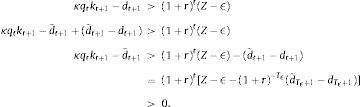
Now consider the following alternative consumption and debt paths whereby we increase consumption in period Tϵ leaving it unchanged in all other periods. We finance this increase in consumption in period Tϵ by issuing debt and then rolling over this additional debt forever. And we leave the path for kt+1 unchanged. We want to know if this alternative path for dt+1 is feasible, that is, satisfies (1)–(3). Let the change in dTϵ+1 be equal to z>0, that is, d˜Tϵ+1=dTϵ+1+z. Then consumption increases in period Tϵ by z/(1+r)>0. This strategy is feasible in period Tϵ, that is, it does not violate the collateral constraint (3), as long as,
We need to show that this new path of debt also does not violate the collateral constraint for any t>Tϵ. The new level of debt in any period t>Tϵ, denoted d˜t+1, can be found by subtracting the sequential budget constraint, Eq. (1), for any period Tϵ+j under the original plan and the alternative plan. Note that for t>Tϵ, ct and kt are the same under the original and alternative plans. This yields:orNow recall from above that for any t≥TϵThe last inequality follows from the assumption that (1+r)−Tϵ(d˜Tϵ+1−dTϵ+1)=(1+r)−Tϵz<Z−ϵ. It follows that (1)–(3) are satisfied under the alternative sequence d˜t+1 and it is hence feasible. Clearly it is associated with higher welfare because consumption in period Tϵ is higher. Therefore, the original sequence could not have been a solution to the household's maximization problem.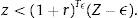


Alternatively, one could assume that borrowing is limited by the expected value of capital at the time debt is due. In this case, the right-hand side of the collateral constraint would be κqt+1kt+1. See, for example, Devereux, Young, and Yu (2015).
We thank for comments Enrique Mendoza and participants at the conference on Policy Lessons and Challenges for Emerging Economies in a Context of Global Uncertainty, organized by the Central Bank of Colombia, Cartagena, Colombia, October 3–4, 2016.
Invited Article.
See, for example, Mendoza (2002, 2005, 2010), Uribe (2006, 2007), Lorenzoni (2008), Jeanne and Korinek (2010), Korinek (2011), Bianchi (2011), and Benigno, Chen, Otrok, Rebucci, and Young (2013, 2014).
In Appendix A we show that if a set of sequences {ct, dt+1, kt+1} satisfies all optimality conditions but (9), then there exists a welfare-dominating set of feasible sequences, that is, sequences satisfying (1)–(3) that generate higher utility.