

En las últimas décadas, se ha presentado una mayor literatura que enfatiza en la capacidad de la banca comercial para aumentar la oferta monetaria a través del crédito y la relación del canal de crédito con el crecimiento económico. En línea con estos planteamientos de teoría económica, este trabajo evalúa la causalidad y los efectos de corto plazo entre el crédito bancario y el crecimiento económico en México a través de la estimación de un modelo de Vectores Autoregresivos (var). Los principales resultados indican que entre 2001Q1 y 2016Q4 el crecimiento del pib tiene causalidad en el sentido de Granger y un efecto positivo sobre la tasa de crecimiento del crédito bancario; sin embargo, no hay evidencia de causalidad o de efecto alguno del crédito bancario sobre el pib. Estos resultados son relevantes y podrían explicarse por factores de oferta y de demanda en el mercado crediticio.
Over the last decades, there has been a growing literature that emphasizes on the capacity of commercial banks to increase the money supply through the act of lending and the relation of the credit channel with the economic growth. Following this economic theory approach, this paper evaluates the causality and the short-term effects between the banking credit and the economic growth in Mexico through the estimation of a Vector Autoregressive (var) model. The main results indicate that from 2001Q1 to 2016Q4 the gdp growth has Granger-caused and a positive effect on the rate of growth of banking credit; however, there is no evidence of causality or any effect of banking credit to the gdp. These results are relevant and could be explained by factors of supply and demand in the credit market.
The financial and the real production sector have been important in the economic analysis due to the implications of finance on the development and the economic growth. Schumpeter (1911) argued that the production decisions are not only taken by entrepreneurs, banks have an important role on its determination as well. Indeed, a virtuous relationship between entrepreneurs and bankers is made at the time that credit goes to finance innovative projects of production (Festré and Nasica, 2009).
Several studies have argued the necessity to strengthen the financial sector in order to promote technological projects that contribute to a higher productivity (Levine, 1997). Moreover, Hicks (1969, pp. 143-145) points out that through economic history the financial sector has been an engine of periods with accelerated paces of production growth, as it was during the industrial revolution. In that period, the innovations in the English financial market contributed to the investment on high technological infrastructure and reduced the risk of illiquidity on economic activity.1
In addition, arguments in favor of financial liberalization promote the free flow of capital from countries which have a saving surplus to those that require investment (Balassa, 1989). For that reason, the lower the transaction costs are, the greater the investment to technological projects in emerging economies would be (Bencivenga, Smith and Starr, 1994). The most important objective of the financial capital is to be used towards its most productive uses.
Some authors argue that credit creation is the main mechanism of the financial system to influence the economic activity, so the approach of credit as a monetary transmission channel has become more relevant in economic theory over the last years. From an institutional view, some researches have proposed that banking credit policies ought to be highly regulated after the crisis of subprime mortgages in the United States.
Clearly, an economy cannot support its long-term growth only by stimulating the credit activity; however, it is important to evaluate the effects of banking credit on economic dynamism in the short-term. The main objective of this paper is to provide a theoretical background and empirical evidence that allows to determine the causality and the short-term effects between the banking credit and the economic growth in Mexico. The distinction between monetary aggregates and banking credit as components of the money supply has allowed economic theorists and researchers to develop different approaches
The organization of this paper is as follows: the first part presents a revision of economic theory that considers an approach of banking credit as a component of the money supply and a channel that leads to macroeconomic effects. The following section shows relevant statistics related to banking credit and macroeconomic variables in Mexico. In the third section, a var (3) model is estimated and gives evidence about the short-term effects and the causality between the gdp and the banking credit growth, both in percentage change quarter to quarter. The last part of this article concludes.
IMacroeconomics and the credit channelThe distinction between monetary aggregates and banking credit as components of the money supply has allowed economic theorists and researchers to develop different approaches about the neutrality and the non-neutrality of money.2
From the orthodox view, the theoretical approaches of the new classical economy and the new Keynesian economy support the idea that changes in the money supply are neutral in the long term, so the economy is totally determined by production factors and is sterile to monetary imbalances (Blanchard, 2006, p. 543). However, the discrepancy between these two approaches relies on the short-term. On the one hand, the new classics affirm that prices are flexible, so variations in the money supply triggers an inflationary process with no effects on production, and thus, the money supply is neutral. On the other hand, the new Keynesians propose that changes in money supply have effects on real variables, due to the rigidities in prices and wages; therefore, the non-neutrality of money implies that an increase of the money supply leads to a rise in both production and aggregate demand (Akerloff and Yellen, 1985).3
During decades, the new Keynesianism had only focused on the monetary aggregates as a transmission channel of monetary policy. Nevertheless, Bernanke and Blinder (1988), Bernanke (1993) and Bernanke and Gertler (1995) investigations switch this focus, they concluded that in practice, the monetary policy uses banking credit as its real transmission channel, so the expansion or the contraction of credit activity affects the economic dynamism.
On the heterodox economics, the Post Keynesian contributions to monetary theory, which are based on Robinson (1956), Kaldor (1970), Minsky (1992), Lavoie (1984) and Moore (1988), emphasized on the concept of a monetary economy of production, due to the fact that the banking sector drives the creation of money through granting loans and is able to stimulate the real sector of production. Thus, the money supply is endogenous and generates fluctuations in production.4
Some other authors such as Graziani (1989), Wray (1990), Parguez and Seccareccia (2000), Rochon (2002), Keen (2009) and Vallageas (2010) developed the Monetary Circuit Theory (mct). This macroeconomic theory gives emphasis to a process of flux and reflux of money between the financial and the real sector of production that generates dynamism in economic activity. Under this approach, the value added is shared between industrial profits and financial gains in order to increase the stock of capital and the financial capital. For that reason, the endogenous creation of money arises from the necessity of the economy to reproduce itself.
According to the Post Keynesian tradition, the endogeneity of money is a concept that describes changes in the money supply through the banking credit. Indeed, some researches support the argument that banks do not simply act as intermediaries between savings and loans; in a modern economy, the banking system has the ability to create money through the act of lending. However, the mechanism of increasing the money supply through the banking credit has its own constraints (McLeay, Radia and Thomas 2014; Tobin, 1964).5
The constraints that banks face in order to grant new credits can be classified as internal or external. The internal constraints refer to those in which the banks are restricted by themselves. In other words, if banks increase their credit supply excessively, this decision leads to diminish their profits and their financial stability. In contrast, the external constraints are those involving the preferences of borrowers (households and firms), financial regulation and monetary policy (McLeay, Radia and Thomas, 2014, p. 17).
Overall, in the last years the economic analysis has emphasized on the banks’ capacity to determine the money supply through the credit channel and to what extent this factor is able to generate changes in economic dynamism.
IIBanking credit in Mexico: stylized factsADefining a proxy of banking credit performanceIn the Mexican credit market, commercial banks’ loan portfolio is a proxy financial variable that measures the performance of the banking credit. The loan portfolio is defined as follows:
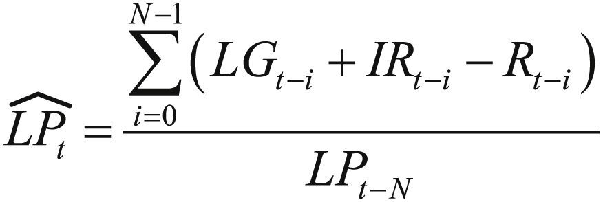
In (1), the banks’ loan portfolio (LP) in the period t is equivalent to the loan portfolio in the previous period (t-1) plus the cash flow between period t and t-1. This cash flow includes the sum of the loans granted (LG) and the interests revenue (IR) minus the debt repayments (DR) in the period t. The rate of growth of (1) is an index that captures the monetary flux and reflux between the banking system and the real sector of production through the loans granted and the debt repayments. The rate of growth in (1) is defined as follows:In (2), N is the number of periods −as the periodicity of LP is quarterly− if N=4, the rate of growth is annual, but, if N=1, the rate of growth is quarter to quarter. In the remainder of this paper, the loan portfolio rate of growth LPˆt is going to be defined as the credit growth crdˆt.BStylized facts of banking credit in Mexico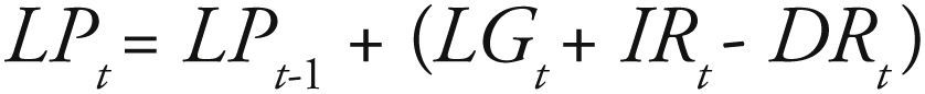
According to data of the National Banking and Securities Commission (cnbv) of Mexico, the most important points to notice about the evolution of the commercial bank loan portfolio are the following:
- •
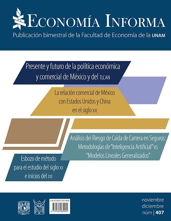
The graph 1a shows that in Mexico the total loan portfolio of commercial banks rose from 1.04 to 4.34 billion of current pesos between 2000Q4 and 2016Q4, in that last quarter, the loan portfolio was equivalent to 20.93% of the Gross Domestic Product (gdp) and this ratio showed a positive trend in the last two years.
- •
The banking loan portfolio is divided in four sectors: firms, households, financial institutions and government. Graph 1b shows the evolution of the loan portfolio percentage composition from 2000Q4 to 2016Q4. Overall, the firms’ and the households’ debt have significantly increased their participation, the government debt decreased and the financial institutions debt increased moderately. During the last quarter of 2016, the firms’ debt was 43.72% of the total, the households’ debt was 37.43%, the government debt was 14.40% and the financial institution debt was 4.45%.6
The loan portfolio and its share of GDP, (1b) the loan portfolio percentage composition by sector in Mexico, 2000Q4-2016Q4. Source: CNBV. Statistical report 040-1A-R0. http://www.cnbv.gob.mx/Paginas/PortafolioDeInformacion.aspx.")
The most relevant results of credit performance in relation to macroeconomic variables are the following:
- •
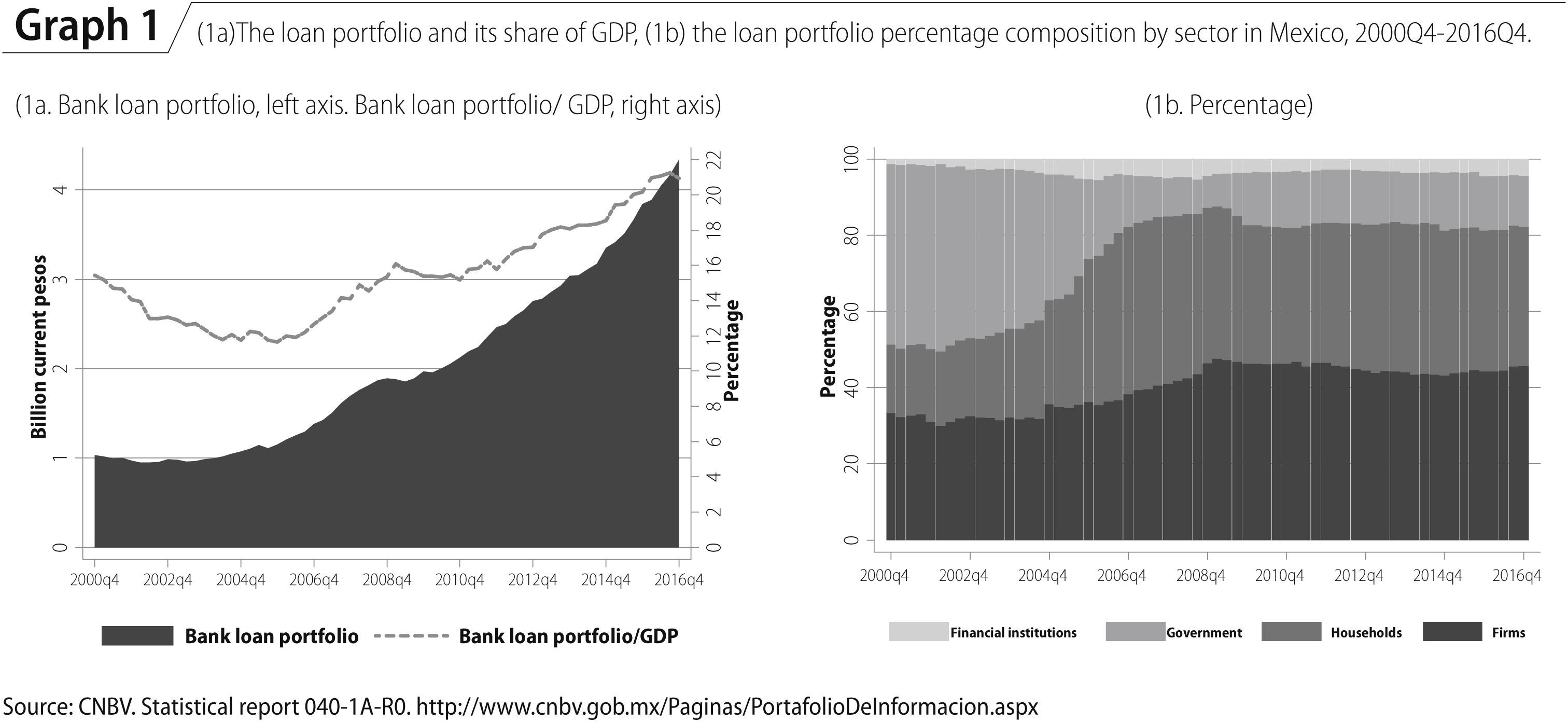
There is a positive association between the gdp annual growth rate and the credit growth, both in real terms; however the credit has a lag of approximately three quarters in relation to the gdp (Graph 2a).7 By sectors, the real gdp growth exhibits a closer correlation with the credit growth to households and firms (Graph 2a). This relation has been deeply studied in recent years for different economies and among countries.8
- •
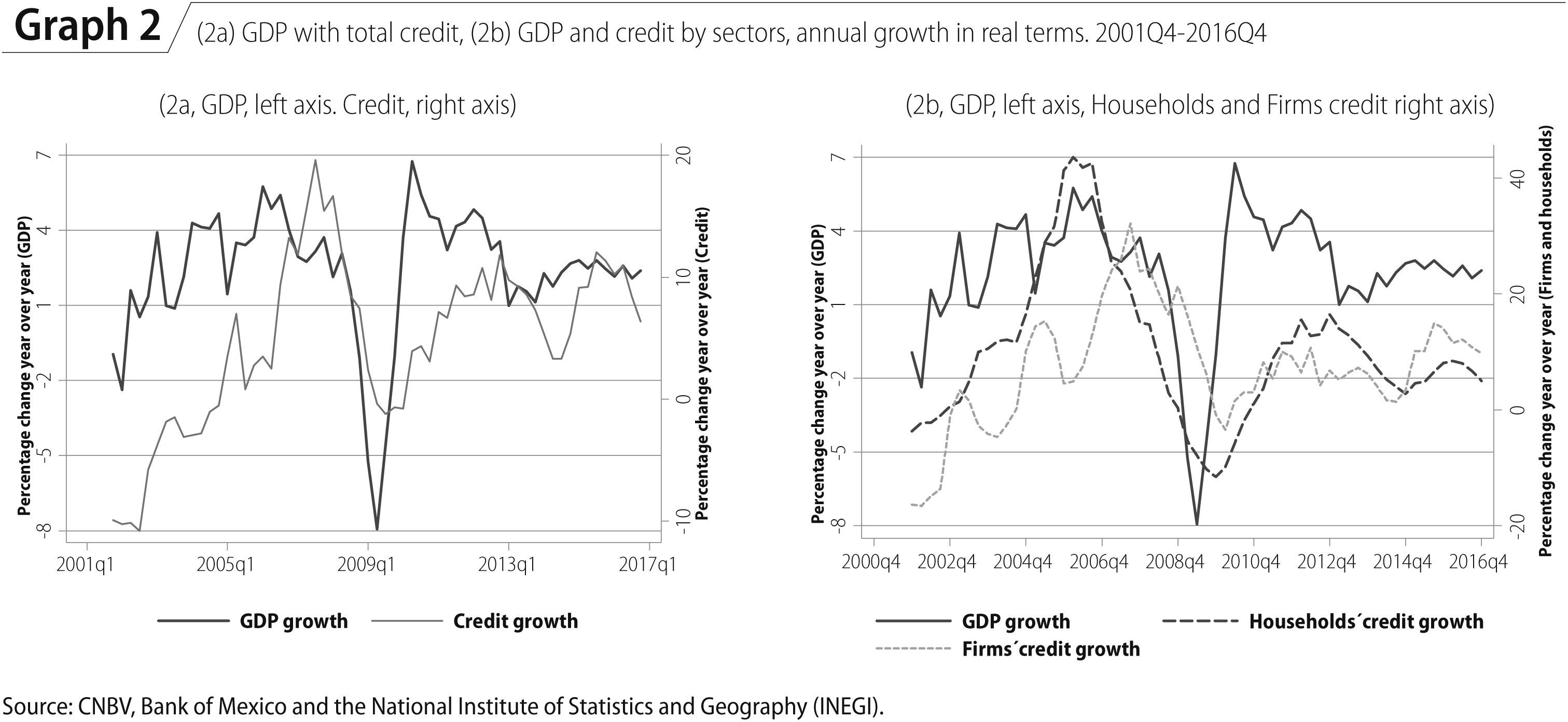
Graph 3a exhibits a weak association between the banking credit growth and the monetary aggregate M2. It could be argued that banking credit remains in greater proportion as electronic money, basically because credit is related to transactions of high value goods such as dwellings, fixed capital and durable goods. In addition, the purchase of goods and services of the consumer basket may be less demanding of this means of payment, so the credit does not appear to have a clear relation with inflation (Graph 3b).
- •
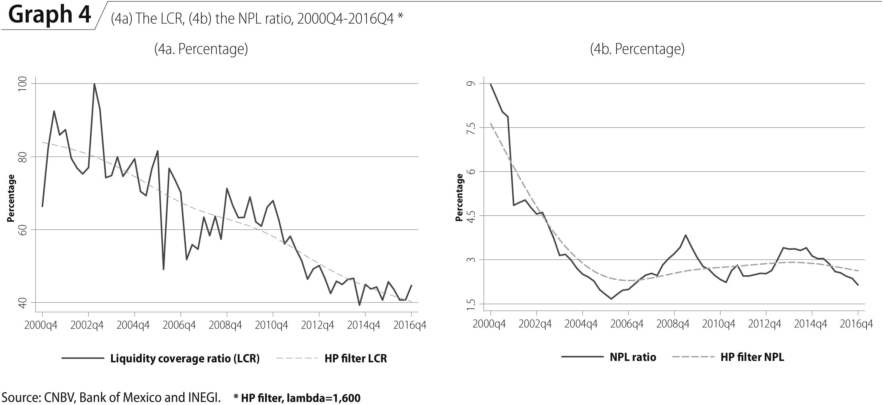
Mexico has adopted Basel III standards that include the risk based capital and the liquidity rules (Basel Committee on Banking Supervision, 2015). For that reason, the Liquidity Coverage Ratio (lcr)9 and the Nonperforming Loan (npl)10 ratio are key variables of banking policy. However, Graph 4a and 4b shows a different path of lcr and npl ratio in relation to the credit growth. In particular, the lcr and the npl ratio exhibits a downward trend and a lower variation in the last two years. As a result, the bank liquidity and the risk of loans in default are not factors that have led to significant changes in credit supply over the recent years.
 GDP with total credit, (2b) GDP and credit by sectors, annual growth in real terms. 2001Q4-2016Q4 Source: CNBV, Bank of Mexico and the National Institute of Statistics and Geography (INEGI).")
 Credit with the monetary aggregate M2, annual growth in real terms, (3b) credit growth and in_ation, 2001Q4 – 2016Q4 Source: CNBV, Bank of Mexico and INEGI.")
 The LCR, (4b) the NPL ratio, 2000Q4-2016Q4 * Source: CNBV, Bank of Mexico and INEGI. * hp filter, lambda=1,600.")
The model estimated in this section is based on a closed economy that captures the causality and the short-term effects between the credit and the gdp. This model is in line with the contemporary econometrics based on a system of dynamic equations (Sims, 1980). The variables included in this analysis are expressed in real terms and deseasonalized with Census X-12. These variables are: the gdp (gdp), and the commercial bank loan portfolio (crd) 11 –as a proxy variable of the banking credit performance– both variables with a quarterly sample from 2000Q4 to 2016Q4.
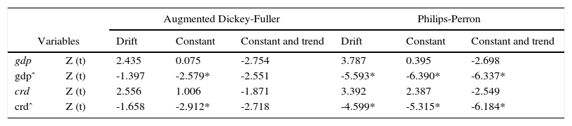
According to the unit root test12 –Philips-Perron (pp)–, the variables in levels are integrated of order one I(1), and their quarter to quarter rate of growth have an order of integration I(0) (Appendix, Table 1).13 For that reason, it is proposed the estimation of a Vector Autoregressive (var) model including the gdpgdpˆ and the banking credit crdˆ, both in rates of growth of quarter to quarter. The Akaike's and the Hannan-Quinn information criteria determine an optimum of three lags in the var model.
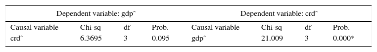
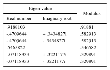
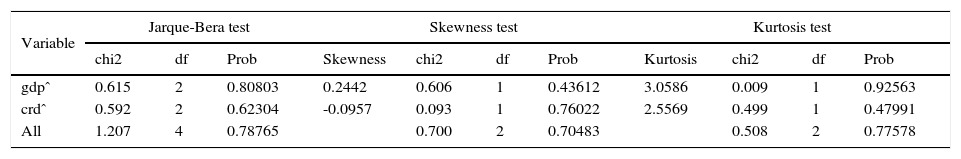
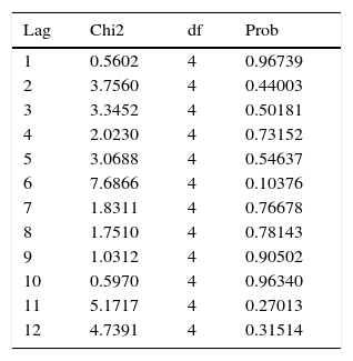
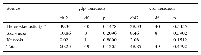
After the var (3) estimation,14 the dynamic stability condition is verified and the diagnostic tests that ensure the appropriate model specification according to the distribution of residuals (Appendix, Tables 2 to 5). One of the most important results of the var model indicates that the gdp growth has causality in the Granger's sense on the banking credit growth. However, there is no causality of the credit growth to the gdp (Table 1). Therefore, the gdp growth is the most exogenous variable in the var model.15
Causality in Granger's sense
| Dependent variable: gdpˆ | Dependent variable: crdˆ | ||||||
|---|---|---|---|---|---|---|---|
| Causal variable | Chi-sq | df | Prob. | Causal variable | Chi-sq | df | Prob. |
| crdˆ | 6.3695 | 3 | 0.095 | gdpˆ | 21.009 | 3 | 0.000* |
H0: Prob>0.05 no causality. Note: *Causality Granger's sense statistically significant Source: Author's calculations.
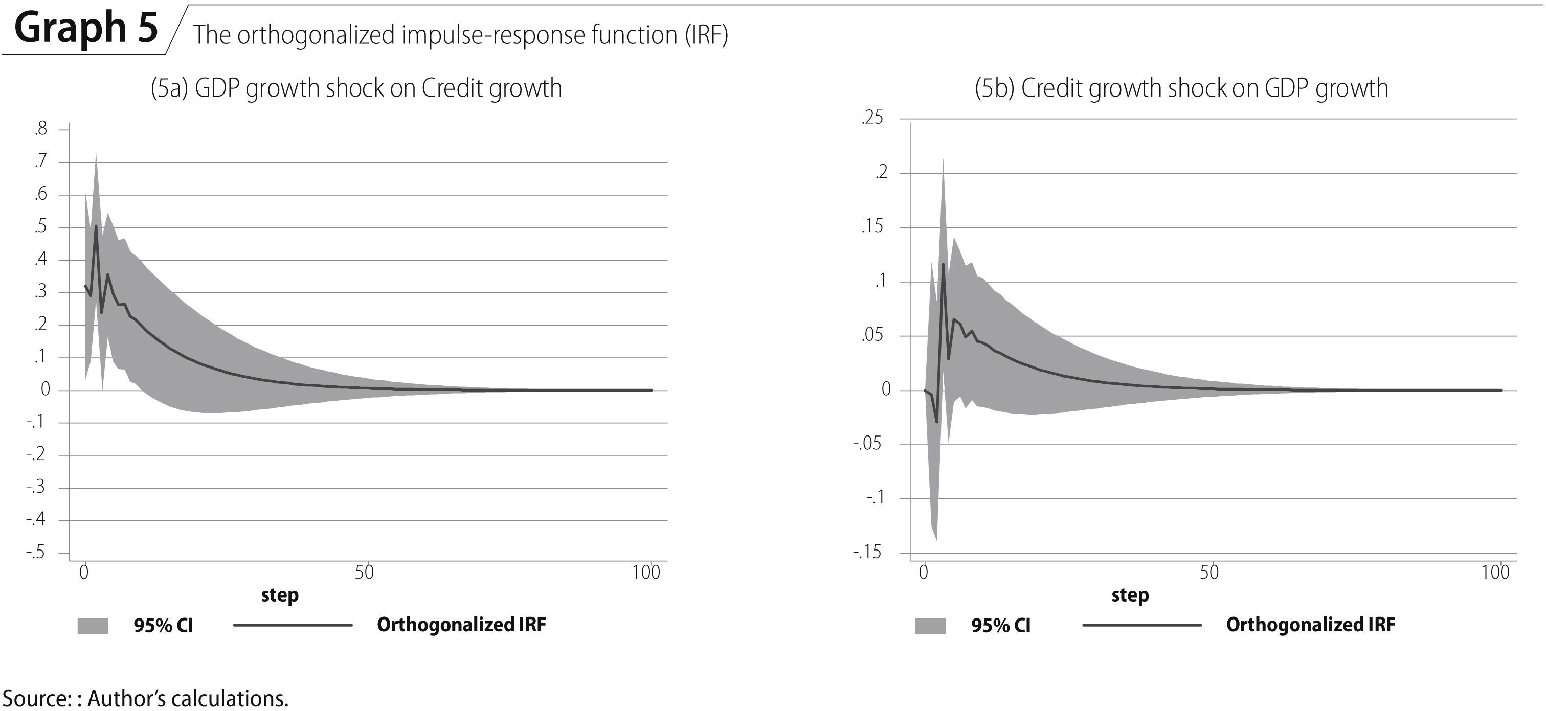
As gdpˆ is the most exogenous variable in the var model according to Granger causality, this is imposed as the first in the ordering of variables. Graph 5 shows the orthogonalized impulse-response function of the model, the most relevant results are the following:
- •
A positive impulse of one standard deviation (SD) in the vector of gdp growth innovations has a statistically significance on the acceleration of the banking credit rate of growth (Graph 5a).
- •
On the other hand, a positive shock in the innovations of the credit growth does not have any effect on the gdp rate of growth (Graph 5b).
 Source: : Author's calculations.")
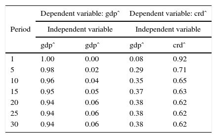
The decomposition of the variance in Table 2 shows that the gdp growth explains itself for the whole period, and after the 10th period, the gdp explains in more than 30% the credit growth. Furthermore, the gdp has an intertemporal capacity to explain itself and the credit growth.
Cholesky decomposition of the variance
| Period | Dependent variable: gdpˆ | Dependent variable: crdˆ | ||
|---|---|---|---|---|
| Independent variable | Independent variable | |||
| gdpˆ | gdpˆ | gdpˆ | crdˆ | |
| 1 | 1.00 | 0.00 | 0.08 | 0.92 |
| 5 | 0.98 | 0.02 | 0.29 | 0.71 |
| 10 | 0.96 | 0.04 | 0.35 | 0.65 |
| 15 | 0.95 | 0.05 | 0.37 | 0.63 |
| 20 | 0.94 | 0.06 | 0.38 | 0.62 |
| 25 | 0.94 | 0.06 | 0.38 | 0.62 |
| 30 | 0.94 | 0.06 | 0.38 | 0.62 |
Source: Author's calculations.
According to the var model results, from 2001Q1 to 2016Q4 the gdp growth has causality in the Granger's sense and has had a positive effect on the rate of growth of banking credit; however, there is no evidence of causality and any effect of banking credit to the gdp. In addition, it is noticeable that the gdp growth is a leading variable that explains the path of growth of the banking credit. These results are relevant and could be explained by factors of supply and demand in the credit market.
On the supply side, the loans granted are a response of the banking expectations about the macroeconomic performance, therefore the gdp growth is a key variable that guides the credit banking policy according to the expectations of income earned by households and firms. Therefore, the gdp growth influence the bank's willingness of lending. This argument is in line with the model of Greenwald and Stiglitz (1991, 1993, 2003) that describes the banks behavior and how they adjust the credit availability and other financial variables not just by conventional monetary instruments but also by the expectations of future constraints.
On the demand side, the banking credit is a mean of payment for households and firms after the production takes place. Therefore, the households’ demand of credit reflects the consumption of newly produced goods and services, particularly dwellings via mortgages, it might be the reason why the credit growth is a lagged variable in relation to the gdp growth. In addition, the firms’ demand of credit can go to the reinvestment of fixed capital and inventory
Unit root test
| Variables | Augmented Dickey-Fuller | Philips-Perron | |||||
|---|---|---|---|---|---|---|---|
| Drift | Constant | Constant and trend | Drift | Constant | Constant and trend | ||
| gdp | Z (t) | 2.435 | 0.075 | -2.754 | 3.787 | 0.395 | -2.698 |
| gdpˆ | Z (t) | -1.397 | -2.579* | -2.551 | -5.593* | -6.390* | -6.337* |
| crd | Z (t) | 2.556 | 1.006 | -1.871 | 3.392 | 2.387 | -2.549 |
| crdˆ | Z (t) | -1.658 | -2.912* | -2.718 | -4.599* | -5.315* | -6.184* |
Note: *Rejecting unit root according to critical values for Dickey–Fuller t-distribution
Source: Author's calculations.
Jarque-Bera test on normality of residuals distribution
| Variable | Jarque-Bera test | Skewness test | Kurtosis test | ||||||||
|---|---|---|---|---|---|---|---|---|---|---|---|
| chi2 | df | Prob | Skewness | chi2 | df | Prob | Kurtosis | chi2 | df | Prob | |
| gdpˆ | 0.615 | 2 | 0.80803 | 0.2442 | 0.606 | 1 | 0.43612 | 3.0586 | 0.009 | 1 | 0.92563 |
| crdˆ | 0.592 | 2 | 0.62304 | -0.0957 | 0.093 | 1 | 0.76022 | 2.5569 | 0.499 | 1 | 0.47991 |
| All | 1.207 | 4 | 0.78765 | 0.700 | 2 | 0.70483 | 0.508 | 2 | 0.77578 | ||
Source: Author's calculations.
Lagrange Multiplier (LM) test for autocorrelation
| Lag | Chi2 | df | Prob |
|---|---|---|---|
| 1 | 0.5602 | 4 | 0.96739 |
| 2 | 3.7560 | 4 | 0.44003 |
| 3 | 3.3452 | 4 | 0.50181 |
| 4 | 2.0230 | 4 | 0.73152 |
| 5 | 3.0688 | 4 | 0.54637 |
| 6 | 7.6866 | 4 | 0.10376 |
| 7 | 1.8311 | 4 | 0.76678 |
| 8 | 1.7510 | 4 | 0.78143 |
| 9 | 1.0312 | 4 | 0.90502 |
| 10 | 0.5970 | 4 | 0.96340 |
| 11 | 5.1717 | 4 | 0.27013 |
| 12 | 4.7391 | 4 | 0.31514 |
Source: Author's calculations.
Cameron & Trivedi's decomposition of Information Matrix (IM-test)
| Source | gdpˆ residuals | crdˆ residuals | ||||
|---|---|---|---|---|---|---|
| chi2 | df | p | chi2 | df | p | |
| Heteroskedasticity * | 49.34 | 40 | 0.1478 | 38.33 | 40 | 0.5455 |
| Skewness | 10.86 | 8 | 0.2096 | 8.46 | 8 | 0.3902 |
| Kurtosis | 0.02 | 1 | 0.8800 | 2.06 | 1 | 0.1512 |
| Total | 60.23 | 49 | 0.1305 | 48.85 | 49 | 0.4792 |
*White's test. Source: Author's calculations.
Maestro en Economía por la unam y profesor adjunto de Teoría Macroeconómica II. Profesionalmente, se desemepeña como analista de estudios económicos y de la vivienda en Sociedad Hipotecaria Federal (shf).
“Liquidity is the ease and speed with which agents can convert assets into purchasing power” (Levine, 1997, p. 692).
The neutrality of money implies that changes in money supply have only effects on nominal variables such as prices, wages or exchange rates without any effect on real variables such as employment, production factors or real gdp.
In addition, monetarism concluded that the money supply leads to short-term oscillations of the business cycle (Friedman and Schwartz, 1986). Particularly, if the increase of the monetary aggregates were higher than the production growth, the inflation would appear as a monetary phenomenon. For that reason, an adequate economic policy is to control the money supply in order to stimulate the economic activity and to maintain the inflationary stability (Friedman, 1960).
Firstly, the banking sector seeks to grant loans, through this mechanism money supply increases, in case of lack of liquidity, bank reserves are obtained in the interbank overnight lending market. There is no reason to suppose that banks maintain a surplus of idle reserves (Holmes, 1969).
Tobin (1964) argued that commercial banks have the ability to create money, however they don’t have the “widow's cruse”. In fact, money created by banks differs from money created by the government, because the governmental sector can use its own resources to finance itself, while the banking sector has to create money to finance other entities.
The firms’ loan portfolio include industrial activities, construction and other productive actions. The households’ loan portfolio includes: loans to consumption (credit card and non-revolving credit) and mortgages. The financial institution debt includes: loans to the banking system and other financial institutions. Finally, the government loan portfolio includes loans to the federal government, to states, to local governments and to other public institutions.
A comparative case of study with this statistic evidence is the regularity of the positive relation between the economic and the credit cycle in Mexico (Herman and Klemm, 2017; Banco de Mexico, 2010) and among different countries (Apostoaie and Percic, 2014, Euopean Banking Federation, 2011). However, credit is not a predictive index to macroeconomic variables, instead, credit cycle is a lagged variable in relation to economic cycle (Bullock, Morris and Steven, 1988, Stevens and Thorp, 1989, Tallman and Chandra, 1996).
Stiglitz (2016) argues that the credit demand can go to increase existing assets such as fixed capital and land.
lcr is the ratio of high liquid assets and net cash outflows
The npl ratio is defined as the relation of the loan portfolio that is in default or close to being in default and the total loan portfolio.
crd is an interchangeable variable definition with lp in equation (1).
Despite the generally accepted practice to use cointegration with non-stationary variables I(1) for estimating a Vector Error Correction (vec), in this case, it was decided not to impose a priori an unidirectional causality constraint on the cointegration vector (Hamilton, 1994, p. 652).
Exogenous variables. Dummy: 2002Q1=1, 2002Q2=-1, 2003Q1=-1, 2004Q1=-1, 2008Q4=1, 2009Q1=1, 2009Q3=1. Dummy2: 2001Q4=1, 2005Q3=1, 2006Q1=-1, 2006Q4=-1, 2007Q2=-1, 2011Q4=1
As it is widely believed, there is no empirical or statistical basis for the choice of the contemporaneous causal ordering in var Model (Demiralp. & Hoover, 2003). However, Granger causality could be a guide.