A Computer Program to Run a Monte Carlo Experiment: A Dickey-Fuller Distribution

Resumen

Se presenta un programa para realizar un experimento de Monte Carlo. Como ejemplo se utiliza una distribución de Dickey-Fuller. Al evitar el uso de matrices el código propuesto es más fácil de ejecutar que el diseñado por, entre otros, Brooks (2002) o Fantazzini (2007). Se presentan algunas notas respecto a la técnica de Monte Carlo y sobre las pruebas de raíces unitarias. Al final se comparan los valores críticos obtenidos con los reportados por Brooks (2002), Charemza and Deadman (1992), Enders (2004), y Patterson (2000).

Abstract

We present a computer program to run a Monte Carlo experiment. We use as example a Dickey-Fuller distribution. Avoiding the use of matrices, the proposed program is easier to put into practice than the code designed by, among others, Brooks (2002) or Fantazzini (2007). Some remarks about the Monte Carlo method and unit root tests are included. At the end we compare our critical values with the ones in Brooks (2002), Charemza and Deadman (1992), Enders (2004), and Patterson (2000).

“But with this miraculous development of the eniac—along with the applications Stan must have been pondering—it occurred to him that statistical techniques should be resuscitated, and he discussed this idea with von Neumann. Thus was triggered the spark that led to the Monte Carlo method.” Nicholas Metropolis (1987, p. 126).

“The obvious implications of these results are that applied econometricians should not worry about spurious regressions only when dealing with I(1), unit root, processes. Thus, a strategy of first testing if a series contains a unit root before entering into a regression is not relevant”. Clive W. J. Granger (2003, p. 560).

1

Unit roots always cause trouble

It came as a bit of shock when econometricians realized that the “t” and the Durbin-Watson statistics did not retain its traditional characteristics in the presence on nonstationary data, i.e. regressions involving unit root process may give non-sense results. Following Bierens (2003), it is correct to say that, if y_t and x_t are mutually independent unit root processes, i.e. y_t is independent of x_t-j for all t and j, then ols regression of y_t on x_t for t=1,…,n, with or without an intercept, will yield a significant estimate of the slope parameter if n is large: the absolute value of the t-value of the slope converges in probability to ∞ if n → ∞. We then might conclude that y_t depends on x_t, while in reality the y_ts are independent of the x_ts. Phillips (1986) was able to show that, in such a case, DW statistic tends to zero. Hence, adding lagged dependent and independent variables would make the misspecified problem worse. By the way, the first simulation on the topic was by Granger and Newbold (1974). They generated two random walks, each one had only 50 terms and 100 repetitions were used! In this sense (Granger, 2003, p. 559), “it seems that spurious regression occurs at all sample sizes.”

How does one test for non-stationarity? In first place a variable is said to be integrated of order d, written I(d), if it must be differenced d times to be made stationary. Thus a stationary variable is integrated of order zero, written I(0), a variable which must be differenced once to become stationary is said to be I(1) integrated of order one, and so on. Economic variables, which include financial ones, are seldom integrated of order greater than two.

Consider the simplest example of an I(1) variable, a random walk without drift. Let y_t = y_t−1 + e_t, where e_t is a stationary error term, i.e., e_t is I(0). Here y_t can be seen to be I(1) because Δy_t = e_t, which is I(0) Now let this relationship be expressed as y_t = ρ*y_t−1 + e_t. If |ρ| < 1, then y is I(0) i.e., stationary, but if ρ = 1 then y_t is I(1), i.e., nonstationary. In this sense, typically formal tests of stationarity are test for ρ = 1, and because of this are referred to as tests for a unit root. By the way, the case of |ρ| > 1 is ruled out as being unreasonable because it would cause the series y_t to explode. In other words, for an I(2) process the remote past is more influential that the recent one, which makes little sense.

In terms of our economics common-sense, the differences between a stationary, or “short memory” variable, and an I(1) or “long memory” one, are clues:

• 1.

  A stationary time series has a mean and there is a tendency for the series to return to that mean, whereas an integrated one tends to wander “widely”.

• 2.

  Stationary variables tend to be “erratic”, whereas integrated variables tend to exhibit some sort of smooth behavior (because of its trend).

• 3.

  A stationary variable has a finite variance, shocks are transitory, and its autocorrelations ρk die out as k grows, whereas an integrated series has an infinite variance, i.e. it grows over time, shocks are permanent, and its autocorrelations tend to one (Patterson, 2000).

2

Monte Carlo simulations

A Monte Carlo experiment attempts to replicate an actual data-generating process (dgp). The process is repeated numerous times so that the distribution of the desired parameters and sample statistics can be tabulated. Its reliability is warranted by the Law of Large Numbers: as the sample size grows sufficiently large, the sample statistic converges to the true one. Thus, the sample statistic is an unbiased estimate of the population one. The beauty of the simulation is that attributes of the constructed series are known to the researcher. It is well-known that a limitation of a Monte Carlo experiment is that the results are specific to the assumptions used to generate the simulated data. For example, if you modify the sample size, include or delete an additional parameter, or use an alternative initial condition, a new simulation needs to be performed.¹

3

An Eviews program to run a Monte Carlo experiment: a Dickey-Fuller distribution

In order to generate a Dickey-Fuller distribution using a Monte Carlo approach, it is necessary to follow four steps:

• 1.

  Generate a sequence of (seudo) random numbers e_t based on a standard normal distribution.²

• 2.

  Generate the sequence y_t = ρ*y_t−1 + e_t (eq. 1), where ρ = 1. With the intention of minimize the influence of y_o, its value is fixed to zero and T = 500.

• 3.

  Estimate the model Δy_t = γ*y_t−1 + e_t (eq. 2), where γ = ρ−1. Following Dickey and Fuller (1979, 1981), the “t” -statistic will be recorded as. Obtain its distribution is our goal. According to Patterson (2000, p. 228), even though γ = 0 by construction, “the presence of e_t a random disturbance term, will prevent us from reaching this conclusion with certainty from a particular dataset”, that is, there will be a distribution of the with nonzero values occurring; if the estimation method is unbiased then this should be picked up if T is large enough “by an average of over the T samples equal to the value in the dgp”. About eq. 2 Charemza and Deadman (1997, p. 99) remind us that, because it is a regression of an I(0) variable on a I(1) variable, “not surprisingly, in such a case the t-ratio does not have a limiting normal distribution.”

• 4.

  Repeat steps 1 to 3. By the way, Dickey and Fuller (1979, 1981) obtained 100 values for e_t, set γ = 1, y₀ = 0 and calculated, accordingly, 100 values for y_t.

The Eviews program to run the experiment is the following:

‘Create a workfile undated, range 1 to 500.

!reps = 50000

for !i = 1 to !reps

genr perturbacion{!i} = @nrnd

smpl 1 1

genr y{!i} = 0

smpl 2 500

genr y{!i} = y{!i}(-1) + perturbacion{!i}

smpl 1 500

matrix(!reps,2) resultados

equation eq{!i}.ls D(y{!i}) = c(1)*y{!i}(-1)

resultados(!i,1) = eq{!i}.@coefs(1)

resultados(!i,2) = eq{!i}.@tstats(1)

d perturbacion{!i}

d y{!i}

d eq{!i}

NEXT

‘Export “resultados” to Excel.

‘Create a workfile undated, range 1 to 50,000.

‘Copy and paste from Excel to the workfile.

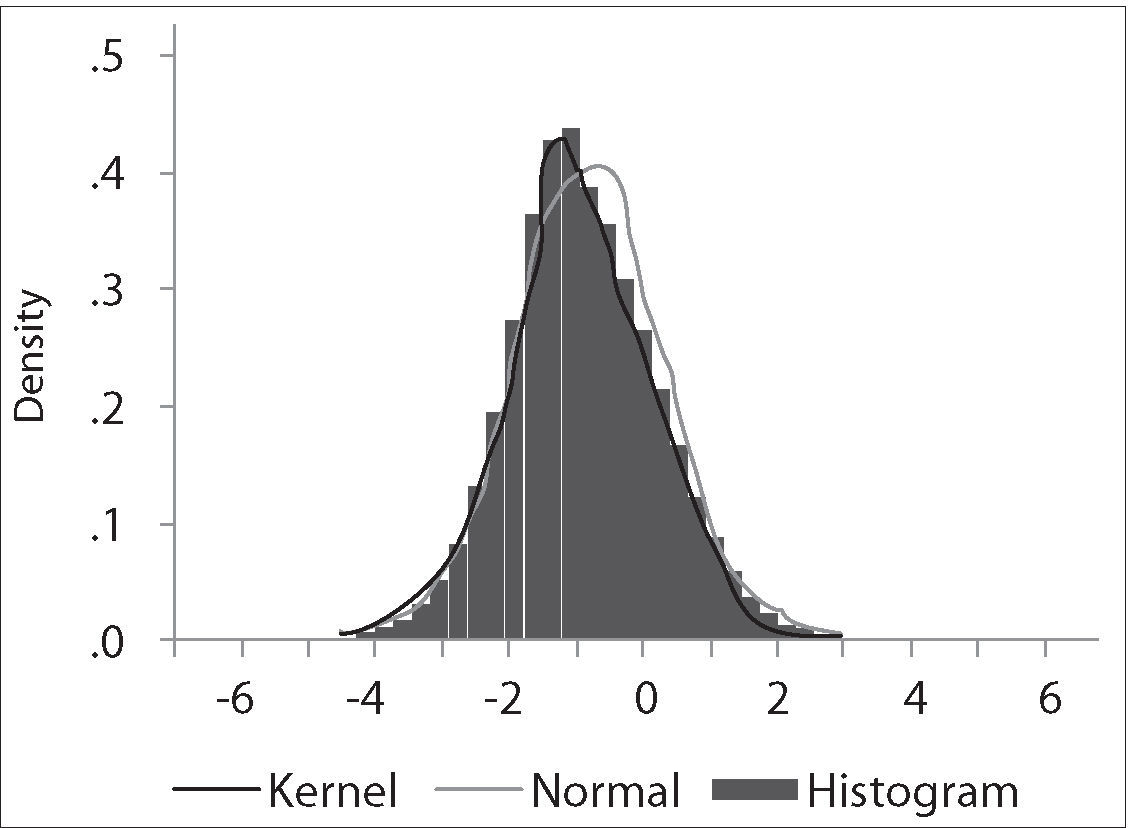
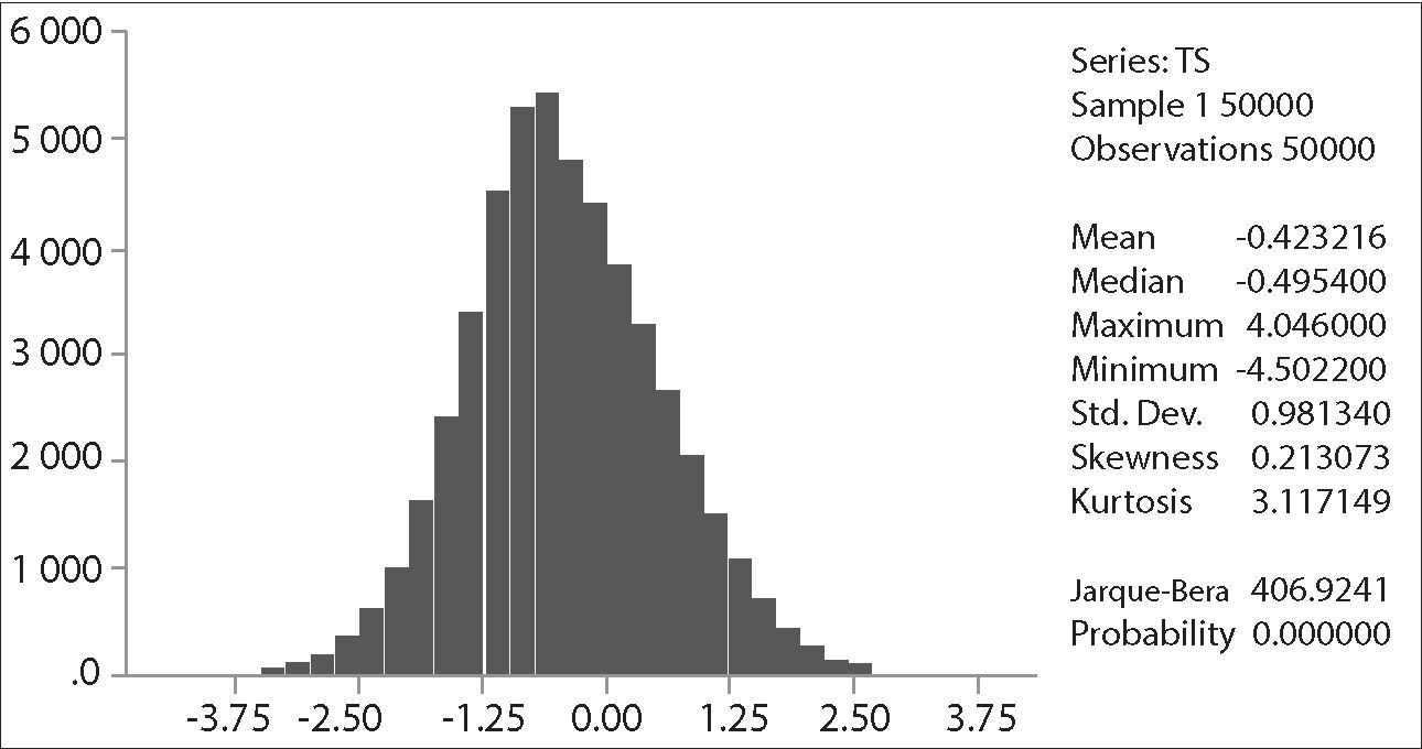
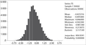
The critical values depend on the specification of the null and alternative hypotheses. The H_o: γ = 0 implying y_t = ρ*y_t−1 + e_t with ρ = 1, that is, y_t ∼ I(1). The alternative “should be chosen to maximize the power of the test in the likely direction of departure from the null. A two-sided alternative γ ≠ 0, comprising γ > 0 and γ < 0 is not chosen in general because γ > 0 corresponds to ρ > 1 and in that case the process generating y_t is not stable; instead the one-side alternative H _a: γ < 0, that is ρ < 1, is chosen because departures from the null are expected to be in this direction corresponding to an I(0) process. Thus the critical values are negative, with sample values more negative than the critical values leading to rejection of the null hypothesis in the direction of the one-side alternative” (Patterson 2000, p. 228). The empirical distribution of our Dickey-Fuller statistic and its descriptive statistics are shown in the following figures:

It is clear that the simulated distribution is not like that of the t-distribution, which is symmetric and centered at zero. In Excel we sort τˆ from the highest values to the lowest ones. The value of −1.9359 is the average between the 2500th and 2501st lowest values in the 50,000 replications, and may be regarded as the critical value at the level of significance of 5%.

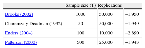
As a final point, in the following table we compare our results with those of Brooks (2002), Charemza y Deadman (1992), Enders (2004), and Patterson (2000).

Table 1.

Critical values, Dickey-Fuller distribution

	Sample size (T)	Replications
Brooks (2002)	1000	50,000	−1.950
Charemza y Deadman (1992)	50	50,000	−1.949
Enders (2004)	100	10,000	−2.890
Patterson (2000)	500	25,000	−1.943

4

Final comments

It is an undeniable true the 3th law in econometrics proposed by Phillips (2003, p. 8), which I borrowed it as the title of the first section: “units roots always cause trouble”. At the moment, you can find not only a good number of papers that propose unit root tests, but also on testing strategies (Perron 1988, Dolado, Jenkinson, and Sosvilla-Rivero 1990, Holden and Perman 1994, Enders 1995, Ayat and Burridge 2000, and Elder and Kennedy 2001). Following Bierens (2003), I recommend the two most frequently applied types of unit root tests, the Augmented Dickey Fuller and the Phillips-Perron tests, and the strategy proposed by Dolado et al. (1990).

Indeed Monte Carlo simulations “have revolutionized the way we approach statistical analysis” (Dufour and Khalaf, 2003, p. 494). We hope that the proposed program, easy to run, and the relevance of the used example, the Dickey-Fuller distribution, both serve as an introduction to the quoted literature.