Exposure to interbank market and risk-taking by Mexican banks

Abstract

Banks can avoid bank runs and panic using the interbank market as a type of coinsurance. Moreover, because of the possibility of losing financial assets, they theoretically have incentives to monitor their peers, borrowing in this market. This paper examines whether bank risks are explained by their exposure to the interbank market. The market discipline hypothesis suggests that bankers are well equipped to monitor their peers, and the interbank borrowing is par excellence an uninsured deposit. Consequently, banks with a larger exposure to the interbank market should present strong bank fundamentals. Using a sample of 37 Mexican banks, from December 2008 to September 2012, and dynamic panel models based on the SYS GMM estimator, I did not find evidence in favor of the market discipline hypothesis. These results are robust to different indicators of bank risk and exposure to interbank markets. This is a wake-up call for policymakers, who should restore market discipline in interbank operations, following the disclosure policy in Basel III.

Resumen

Los bancos pueden evitar las huidas y el pánico utilizando el mercado interbancario como un tipo de coseguro. Además, debido a la posibilidad de perder activos financieros, teóricamente tienen incentivos para supervisar a sus homólogos, solicitando préstamos en este mercado. Este artículo examina si los riesgos bancarios se explican mediante su exposición al mercado interbancario. La hipótesis de disciplina de mercado sugiere que los banqueros están bien equipados para supervisar a sus homólogos, y los préstamos interbancarios son, por excelencia, depósitos no asegurados. Por tanto, los bancos con una mayor exposición al mercado interbancario deben presentar sólidos fundamentos bancarios. Utilizando una muestra de 37 bancos mexicanos, de diciembre de 2008 a septiembre de 2012, y modelos dinámicos con datos de panel, basados en el estimador SYS GMM, no se encontró una evidencia a favor de la hipótesis de disciplina de mercado. Estos resultados son robustos con respecto a diferentes indicadores de riesgo bancario y de exposición a los mercados interbancarios. Suponen una llamada de advertencia para los legisladores, quienes deben restaurar la disciplina de mercado en las operaciones interbancarias, como continuación de la política de divulgación de información de Basilea III.

1

Introduction

In banking markets, economic agents should respond to bank risk-taking because their costs have a direct relationship with bank risk. This response is known as the market discipline hypothesis, which is a major recommendation in Basel III for the soundness of banking systems and financial development, with a specific relevance in times of the financial globalization (Ayadi, 2013; Basel Committee on Banking Supervision, 2013; Tovar-García, 2011a,b).

This hypothesis has been extensively tested in the subordinated debt market (Evanoff et al., 2011; De Mendonça and Villela Loures, 2009; Tovar-García, in press), in the retail deposit market (Tovar-García, 2014; Berger and Turk-Ariss, 2014), and even in the loan market (Tovar-García, 2012b; Kim et al., 2005). The major findings suggest that the bank's creditors discipline their banks by means of three mechanisms: price, quantity, and maturity. For instance, depositors request higher interest rates from riskier banks, or they can withdraw their deposits, or shift their financial assets from long- to short-term. These reactions have been confirmed in Latin American countries, for Chile, Argentina and Mexico during the 90s (Martinez-Peria and Schmukler, 2001), in Venezuela (Muñoz et al., 2013), in Colombia (Márquez, 2011), and several other countries in different periods (Tovar-García, 2014).

In particular, market discipline is well supported by uninsured depositors, and interbank borrowing is considered par excellence as an uninsured deposit. Accordingly, this market should respond strongly to excessive bank risk-taking. However, the theory is ambiguous and the empirical evidence on market discipline in interbank markets is still scarce. Given this, the present research is motivated by the following question: do banks with larger exposure to interbank markets show lower bank risk?

If the answer is positive, we can interpret this finding as evidence for discipline in the interbank market induced by peers. This test has been explored in Central and Eastern European countries (Dinger and Von Hagen, 2009; Distinguin et al., 2013) and in the Netherlands (Liedorp et al., 2010). Thus, the focus of this research is on the bank risk-exposure nexus. Note that this article does not attempt to test the mechanisms of market discipline in the interbank market (price, quantity, and maturity), which have been tested in USA (Furfine, 2001; King, 2008), Portugal (Cocco et al., 2009), Italy (Angelini et al., 2009), and Russia (Semenova and Andrievskaya, 2012).

The interbank market also can be a channel to transmit risks (Allen and Gale, 2000; Freixas et al., 2000). In the Dutch case, the empirical evidence contradicts the market discipline hypothesis and supports the contagion hypothesis (Liedorp et al., 2010). In Latin American countries the market discipline hypothesis in the interbank market has not been tested. Mexico is an interesting case because its banking system has been expropriated in 1982 due to the debt crisis, privatized in 1991 and bailed out in 1997 soon after the so-called Tequila crisis in 1994–1995. In addition, recent findings suggest a weak discipline induced by Mexican depositors, debt holders, and borrowers (Tovar-García, 2012b, 2014, in press).

Consequently, this research contributes to the empirical literature in three ways. First, this is the first time that the bank risk-exposure nexus is tested in Mexico. Second, it uses a large range of dependent and independent variables to check robustness. Third, it employs panel data in a dynamic model with a SYS GMM estimator (generalized method of moments) that has not been used before to test discipline in the interbank market.

The rest of the paper is organized as follows. Section 2 reviews the literature on market discipline in the interbank market. Section 3 describes the data set, a sample of 37 Mexican banks over the period from December 2008 to September 2012. Section 4 specifies econometric models and reports and discusses the results. Finally, conclusions, recommendations and proposals for future research are outlined.

2

Literature review

“Bankers are especially familiar with the business of banking and therefore have a comparative advantage in determining whether a run on another bank was called for” (Calomiris and Kahn, 1991: 773). In addition, banks have incentives to monitor borrowers (in this case other banks) because of the probability of losing money. Thanks to monitoring activities is possible to minimize losses, and the informed bank will be able to claim debt and escape first than others uninformed bank creditors. Nevertheless, interbank relationships are complex, and banks can avoid bank runs and panic using the interbank market as a type of coinsurance. This market can function in favor of cooperation and coordination in the payment system, especially in times of financial stress (Calomiris and Kahn, 1996).

The interbank market helps banks with liquidity problems, borrowing to balance its payments, and usually this is for a very short-term financing. Consequently, the lending bank can quickly escape from monitoring tasks. Nevertheless, in modern interbank relationships these operations are reiterated, have grown considerably, and are shifting from the overnight to medium and long-term. These new characteristics motivate peer monitors to obtain economic information with a larger perspective about the borrower's financial position.

Rochet and Tirole (1996) state that the peer monitoring can regulate the risky behavior of the borrowing bank, but it can be effective only under correct incentives: the lending bank must feel at risk and must be formally responsible of losses due to its decisions in banking markets. The monetary authority must not rescue each bank in troubles, sending clear signals to the market.

Private lenders in the interbank market cannot distinguish solvent banks in times of financial stress, liquidity shocks, and uncertain about techniques and judgments on risk-taking by peers. Consequently, the government intervention is preferable, yet this implies that the government intervention (as protection) is an amplifier of risk-taking by banks (Flannery, 1996).

The experience suggests that the financial sector is very susceptible, particularly in times of the financial globalization, and a small shock in one or a few banks is able to spread by contagion to the entire economy, in one or several countries, negatively impacting the processes of financial development (Tovar-García, 2011a,b, 2012a). The interbank market is clearly a channel for contagion. Thus, we found that the interbank market is a place where the peer monitoring can function, but also this market is a channel for contagion (Allen and Gale, 2000; Freixas et al., 2000).

Empirically, the literature explores whether banks with more exposure to the interbank market have lower levels of bank risk (the bank risk-exposure nexus). The baseline model to test this nexus can be written as (1):

where the dependent variable is a measure of bank risk, and the key explanatory variable is a measure of the individual bank exposure to the interbank market, principally as borrower. X represents control variables. Dinger and Von Hagen (2009), Distinguin et al. (2013) and Liedorp et al. (2010) are the main works testing the bank risk-exposure nexus.

Dinger and Von Hagen (2009) and Distinguin et al. (2013) study a sample of Central and Eastern European countries, they find evidence in favor of the market discipline hypothesis where the interbank exposure result in lower risk of the borrowing banks. On the contrary, in the Dutch case, Liedorp et al. (2010) do not find evidence in favor of the peer monitoring hypothesis. Their findings suggest that larger shares of both interbank lending and borrowing increase the risk-taking of financial institutions, supporting the contagion hypothesis.¹

Nier and Baumann (2006) examine a similar relationship between capital buffers and interbank deposits, and their findings indicate that a larger proportion of interbank deposits creates incentives for banks to limit their risk of insolvency, by choosing a larger capital buffer for given risk. Other scholars study the mechanisms of market discipline, whether riskier banks pay higher borrowing interest rates and/or receive less credit in the interbank market. In USA, the empirical evidence suggest that high-quality banks, that is, with higher profitability, higher capital ratios, and fewer bad loan problems, pay lower interest rates when they borrow in the interbank market, and riskier banks are less likely to use these loans as a source of liquidity (Furfine, 2001; King, 2008). Similar findings were found in the Portuguese and Italian interbank market (Cocco et al., 2009; Angelini et al., 2009). In Russia, banks with higher capital adequacy ratios enjoy lower interest rates (Semenova and Andrievskaya, 2012). These are related concerns, but outside of the limits of the present research.

3

Data and descriptive statistics

Following Tovar-García (2012b, 2014), the data used in this research are drawn from the historical statistics of the National Banking and Securities Commission (known by its Spanish acronym, CNBV), covering the period 2000–2012. Although CNBV reports monthly statistics, I use quarterly data due to the quarterly nature of the bank variables. In addition, because of lack of information for several banks and periods I analyze only 37 banks over the years 2008–2012, after the failure of Lehman Brothers. I expect that the bankers were very predisposed to monitor bank risk during these crisis years, because of the wake-up call (Martinez-Peria and Schmukler, 2001).

3.1

Measures of bank risk and interbank exposure

I use the Z-SCORE, as dependent variable, to test the bank risk-exposure nexus. It is defined as the 3-year average of the 12 month return on assets (ROA) plus the 3-year average ratio capital to total assets (CAPITALR), divided by the 3-year standard deviation of ROA. This indicator has been extensively employed in the literature to capture the bank risk of insolvency, and to test the market discipline hypothesis in the interbank market (Distinguin et al., 2013; Liedorp et al., 2010). A higher Z-SCORE value indicates a lower probability of bank failure, that is, low-risk bank.

In addition, as measure of bank risk, I employ the reserve for loan losses (RESERVE) defined as the balance at quarter end of provisions for possible credit losses divided by nonperforming loans. A higher RESERVE value indicates a lower probability of bank failure. Similarly, with an inverse relationship with bank risk, I employ nonperforming loans divided by total loans (DOUBTFUL). Dinger and Von Hagen (2009) employ similar variables to measure bank risk.

The key explanatory variable of bank risk is the participation in the interbank market, as a lender or borrower. I employ four variables to measure this participation. First, the ratio of interbank lending to total assets (EXPOSURE1). Second, the ratio of interbank borrowing to total assets (EXPOSURE2). Third, the ratio of interbank borrowing to total deposits (EXPOSURE3). Finally, the ratio of net interbank assets (interbank lending minus interbank borrowing) to total assets (EXPOSURE4). In the former variable, note that negative values indicate that the bank is a net borrower.²

I expect that banks with higher exposure to the interbank market, especially as borrowers, will have lower levels of bank risk. Then, higher values of EXPOSURE1–3 and lower values of EXPOSURE4 should impact positively reducing the bank risk-taking.

Former studies employed measures of the CAMEL rating system (capital adequacy, asset quality, management, earnings and liquidity) to control the effect of EXPOSURE. It is worth noting that the CAMEL indicators frequently are used to capture the bank risk (Tovar-García, 2014).

In this research, capital adequacy is measured with the ratio of capital to total assets (CAPITALR). For asset quality, I use the reserve for loan losses (RESERVE) and nonperforming loans (DOUBTFUL). For management quality, the ratio 12 month managerial expenses to annual average total assets (MANAGEMENT1) and the ratio 12 month managerial expenses to 12 month total income (MANAGEMENT2). Earnings are captured with the 12 month return on assets (ROA) and the 12 month return on capital (ROE). For liquidity, I use the ratio short-term (circulating) assets to total assets (LIQUIDITY1) and the ratio short-term assets to short-term liabilities (LIQUIDITY2).

According to findings in previous empirical studies, bank size is a relevant explanatory variable. Consequently, I approach the size effect using the logarithm of total assets (SIZE), and I analyze bank subsamples.

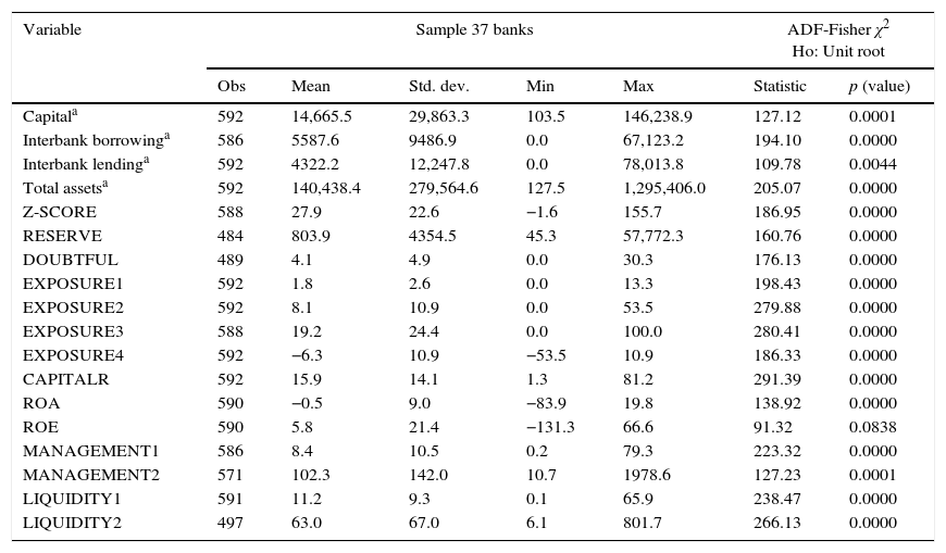
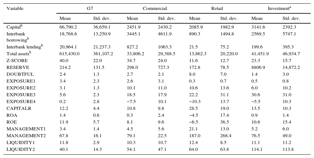
3.2

Descriptive statistics and subsamples of banks

The summary statistics of the variables can be seen in Tables 1 and 2. As a first step, I reviewed the data to eliminate outliers. I use four subsamples of banks, following the classification of Banxico, as Tovar-García (2012b, 2014). The first subsample includes seven of the largest banks (G7), which usually are a cutoff point in the reports of Banxico. In September 2012, the G7 operated around 92% of interbank lending and around 62% of interbank borrowing. The second subsample includes 14 commercial banks with typical activities, but smaller than the G7. The third subsample includes 9 retail banks, which specialize in transactions with consumers. Finally, the fourth subsample includes seven investment banks, working on the issuance of securities.

Table 1.

Descriptive statistics and panel unit root test of the variables for Mexican banks (2008–2012).

Variable	Sample 37 banks					ADF-Fisher χ^2 Ho: Unit root
	Obs	Mean	Std. dev.	Min	Max	Statistic	p (value)
Capital^a	592	14,665.5	29,863.3	103.5	146,238.9	127.12	0.0001
Interbank borrowing^a	586	5587.6	9486.9	0.0	67,123.2	194.10	0.0000
Interbank lending^a	592	4322.2	12,247.8	0.0	78,013.8	109.78	0.0044
Total assets^a	592	140,438.4	279,564.6	127.5	1,295,406.0	205.07	0.0000
Z-SCORE	588	27.9	22.6	−1.6	155.7	186.95	0.0000
RESERVE	484	803.9	4354.5	45.3	57,772.3	160.76	0.0000
DOUBTFUL	489	4.1	4.9	0.0	30.3	176.13	0.0000
EXPOSURE1	592	1.8	2.6	0.0	13.3	198.43	0.0000
EXPOSURE2	592	8.1	10.9	0.0	53.5	279.88	0.0000
EXPOSURE3	588	19.2	24.4	0.0	100.0	280.41	0.0000
EXPOSURE4	592	−6.3	10.9	−53.5	10.9	186.33	0.0000
CAPITALR	592	15.9	14.1	1.3	81.2	291.39	0.0000
ROA	590	−0.5	9.0	−83.9	19.8	138.92	0.0000
ROE	590	5.8	21.4	−131.3	66.6	91.32	0.0838
MANAGEMENT1	586	8.4	10.5	0.2	79.3	223.32	0.0000
MANAGEMENT2	571	102.3	142.0	10.7	1978.6	127.23	0.0001
LIQUIDITY1	591	11.2	9.3	0.1	65.9	238.47	0.0000
LIQUIDITY2	497	63.0	67.0	6.1	801.7	266.13	0.0000

Source: Author's calculations using CNBV data.

a

Balances at quarter end, in millions of Mexican pesos; the rest of variables are ratios in percent, excepting Z-SCORE.

Table 2.

Descriptive statistics of the variables for Mexican banks by subsamples (2008–2012).

Variable	G7		Commercial		Retail		Investment^a
	Mean	Std. dev.	Mean	Std. dev.	Mean	Std. dev.	Mean	Std. dev.
Capital^b	66,790.2	36,659.1	2451.9	2430.2	2085.9	1982.9	3141.6	2392.3
Interbank borrowing^b	18,768.6	13,250.9	3445.1	4611.9	890.3	1494.8	2569.5	5747.1
Interbank lending^b	20,964.1	21,237.3	827.2	1063.3	21.5	75.2	199.6	395.3
Total assets^b	615,430.0	361,107.2	33,806.2	29,388.5	13,862.3	20,220.0	41,451.9	46,934.7
Z-SCORE	40.0	22.0	34.7	24.0	11.6	12.7	23.3	15.7
RESERVE	214.2	131.5	298.0	727.3	172.8	78.5	8806.9	14,872.2
DOUBTFUL	2.4	1.3	2.7	2.1	8.0	7.0	1.4	3.0
EXPOSURE1	3.4	2.3	2.6	3.1	0.3	0.7	0.5	0.8
EXPOSURE2	3.1	1.3	10.1	11.0	10.6	13.6	6.0	10.2
EXPOSURE3	5.6	2.3	18.5	17.9	22.2	31.1	30.6	31.0
EXPOSURE4	0.2	2.8	−7.5	10.1	−10.3	13.7	−5.5	10.3
CAPITALR	12.2	4.4	10.8	9.8	28.5	19.0	13.5	10.3
ROA	1.4	0.6	0.3	2.4	−4.5	17.4	0.9	1.4
ROE	11.9	5.7	8.1	9.6	−6.5	36.5	10.6	15.4
MANAGEMENT1	3.4	1.4	4.5	5.6	21.1	13.0	5.2	6.0
MANAGEMENT2	67.8	16.1	79.1	22.5	187.0	268.4	76.5	49.0
LIQUIDITY1	11.8	2.9	10.3	10.7	12.4	8.5	11.1	11.2
LIQUIDITY2	40.1	14.3	54.1	47.1	64.0	63.8	114.1	113.8

G7: Banamex, Banorte, BBVA Bancomer, HSBC, Inbursa, Santander, and Scotiabank.

Retail banks: American Express, Autofin, Banco Azteca, Bancoppel, Compartamos, Banco Fácil, Banco Ahorro Famsa, Volkswagen Bank, and Banco Wal-Mart.

Commercial banks: ABC Capital, Afirme, Banco del Bajío, Banregio, Bansí, CIBanco, Interacciones, Inter Banco, Invex, Ixe, Banca Mifel, Multiva, Bank of Tokyo-Mitsubishi Ufj, and Ve por Más.

Investment banks: Actinver, Bank of America, Deutsche Bank, ING, JP Morgan, Monex, and Royal Bank of Scotland.

Source: Author's calculations using CNBV data.

a

RESERVE and DOUBTFUL include only information of Monex and Royal Bank of Scotland.

b

Balances at quarter end, in millions of Mexican pesos; the rest of variables are ratios in percent, excepting Z-SCORE.

Mexican banks present a large dispersion of their characteristics, according to the standard deviations of the bank variables. However, this dispersion diminishes considerably in the bank subsamples. On average, the seven largest banks are around 30 times larger (by total assets) than the rest of banks, and these differences are also appreciable in terms of capital.

The largest proportion of interbank lending and borrowing correspond to the G7, on average, they are net lenders. Conversely, other kinds of banks are net borrowers, especially retail banks, as can be observed in the values of the variable EXPOSURE4. The interbank deposits are more relevant for investment banks than for the rest of banks, as we can expect, because non-investment banks have better positions in the retail deposit market (see EXPOSURE3 in Table 2). The participation as lender in the interbank market is relevant for the G7 and commercial banks (see EXPOSURE1 in Table 2), and the participation as borrower in the interbank market is not relevant for the G7 in comparison to other types of banks (see EXPOSURE2 in Table 2).

On average, Z-SCORE (measure of bank risk) equals 27.9, the G7 and commercial banks are above the mean, that is, they are banks with a low-risk. Conversely, retail and investment banks are below the mean, as we can expect, because of the nature of their portfolios. Investment banks show better positions in the variables RESERVE and DOUBTFUL, but this result must be treated with caution because the sample include only two investment banks, and they have the largest values.

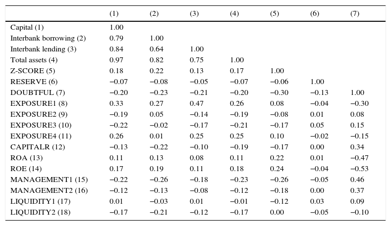
The correlation matrix (see Table 3) shows relevant positive relationships among total assets, capital, and the amount borrowed in the interbank market. These correlations are in line with previous findings about the relevance of the largest banks in the interbank transactions. The measures of exposure to the interbank market show high correlations among EXPOSURE2, 3 and 4, as might be expected, but they show a low correlation with EXPOSURE1, that is, the position as a lender in the interbank market has a low correlation with the position as borrower. The CAMEL indicators present some high correlations among them. Subsequently, in the regression analysis these variables are included with prudence, to avoid multicollinearity concerns. It is noteworthy that I can use these high correlations to check robustness of the results to different indicators of the theoretical variables.

Table 3.

Correlation matrix (pairwise).

	(1)	(2)	(3)	(4)	(5)	(6)	(7)
Capital (1)	1.00
Interbank borrowing (2)	0.79	1.00
Interbank lending (3)	0.84	0.64	1.00
Total assets (4)	0.97	0.82	0.75	1.00
Z-SCORE (5)	0.18	0.22	0.13	0.17	1.00
RESERVE (6)	−0.07	−0.08	−0.05	−0.07	−0.06	1.00
DOUBTFUL (7)	−0.20	−0.23	−0.21	−0.20	−0.30	−0.13	1.00
EXPOSURE1 (8)	0.33	0.27	0.47	0.26	0.08	−0.04	−0.30
EXPOSURE2 (9)	−0.19	0.05	−0.14	−0.19	−0.08	0.01	0.08
EXPOSURE3 (10)	−0.22	−0.02	−0.17	−0.21	−0.17	0.05	0.15
EXPOSURE4 (11)	0.26	0.01	0.25	0.25	0.10	−0.02	−0.15
CAPITALR (12)	−0.13	−0.22	−0.10	−0.19	−0.17	0.00	0.34
ROA (13)	0.11	0.13	0.08	0.11	0.22	0.01	−0.47
ROE (14)	0.17	0.19	0.11	0.18	0.24	−0.04	−0.53
MANAGEMENT1 (15)	−0.22	−0.26	−0.18	−0.23	−0.26	−0.05	0.46
MANAGEMENT2 (16)	−0.12	−0.13	−0.08	−0.12	−0.18	0.00	0.37
LIQUIDITY1 (17)	0.01	−0.03	0.01	−0.01	−0.12	0.03	0.09
LIQUIDITY2 (18)	−0.17	−0.21	−0.12	−0.17	0.00	−0.05	−0.10

	(8)	(9)	(10)	(11)	(12)	(13)	(14)
EXPOSURE1 (8)	1.00
EXPOSURE2 (9)	0.14	1.00
EXPOSURE3 (10)	−0.09	0.71	1.00
EXPOSURE4 (11)	0.10	−0.97	−0.74	1.00
CAPITALR (12)	−0.23	0.13	0.19	−0.18	1.00
ROA (13)	0.12	0.04	0.01	−0.01	−0.43	1.00
ROE (14)	0.14	−0.02	−0.03	0.06	−0.45	0.89	1.00
MANAGEMENT1 (15)	−0.29	0.10	0.12	−0.16	0.68	−0.44	−0.39
MANAGEMENT2 (16)	−0.13	0.12	0.09	−0.15	0.39	−0.74	−0.66
LIQUIDITY1 (17)	−0.03	−0.06	0.00	0.05	0.17	0.03	0.05
LIQUIDITY2 (18)	−0.11	−0.06	0.06	0.03	0.17	0.08	0.08

	(15)	(16)	(17)	(18)
MANAGEMENT1 (15)	1.00
MANAGEMENT2 (16)	0.51	1.00
LIQUIDITY1 (17)	0.25	0.02	1.00
LIQUIDITY2 (18)	0.04	−0.06	0.25	1.00

Source: Author's calculations using CNBV data.

4

Empirical strategy

This research uses regression analysis, as previous tests on market discipline. Note that the dependent and independent variables might face endogeneity concerns. Therefore, it is necessary to use instrumental variables, a difficult task due to data limitations. Furthermore, we are analyzing relations with past dependence, that is, the bank risk of yesterday can be a good forecast of the current bank risk. Testing the asset side of market discipline, Tovar-García (2012b) exploits these characteristics among dependent and independent variables, and recommends dynamic panel data models.

The SYS GMM estimator (Blundell and Bond, 1998) allows for lagged values of the dependent variable to be entered as regressors, and it uses lags of independent variables in first differences and in levels as instrumental variables to correct endogeneity. It is assumed that the error term is not serially correlated and Sargan's over-identification test is employed to validate the instruments.

King (2008) and Semenova and Andrievskaya (2012) to test the market discipline hypothesis in the interbank market used a Heckman correction because some banks do not participate in the interbank market, and it is necessary to control for real-zero exposure. A Heckman model is appropriate for markets with many banks, where is complicated to know if a bank, often a small bank, really is not operating in the interbank market. Certainly, it is better to use a proxy of the probability of exposure.

In the Mexican case, there are a few banks, and all of them are usually participating in the interbank market. In interludes, some banks do not borrow or lend in this market, but we can trust that this is a real-zero exposure for a specific period.

4.1

The bank risk-exposure nexus

Eq. (2) is used to test the bank risk-exposure nexus. The SYS GMM method is alleviating possible endogeneity concerns, and I lag the explanatory variables by one quarter and include a logarithmic transformation of some variables to achieve linearity and semi-elasticity coefficients.

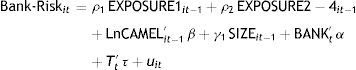
Bank-Risk can be Z-SCORE, RESERVE or DOUBTFUL, the key explanatory variable is EXPOSURE. It is not possible to enter all the measures of exposure at the same time because of collinearity. Consequently, I include EXPOSURE1 in combination with EXPOSURE2, 3 or 4. LnCAMEL includes, in logarithms, combinations of the indicators of capital adequacy, asset quality, management, earnings and liquidity (taking into account collinearity concerns among them).³ SIZE is controlling bank size and BANK is a dummy variable for each type of bank (G7, commercial, retail and investment), where the G7 is the reference group. Thus, the model controls for other bank characteristics and markets. T is a dummy variable for years⁴ controlling effects of unspecified macroeconomic and financial market conditions, which are assumed constant across banks.

The fundamental hypothesis of interest is that bank risk is lower for banks with a higher participation in the interbank market. Z-SCORE and RESERVE depend positively upon the level of EXPOSURE1–3 and inversely upon the level of EXPOSURE4, considering that interbank borrowing is the major channel to mitigate the risk-taking. On the contrary, DOUBTFUL depends inversely upon of the level of EXPOSURE1–3 and positively upon the level of EXPOSURE4. This is interpreted as evidence for market discipline induced by other banks in the interbank market.

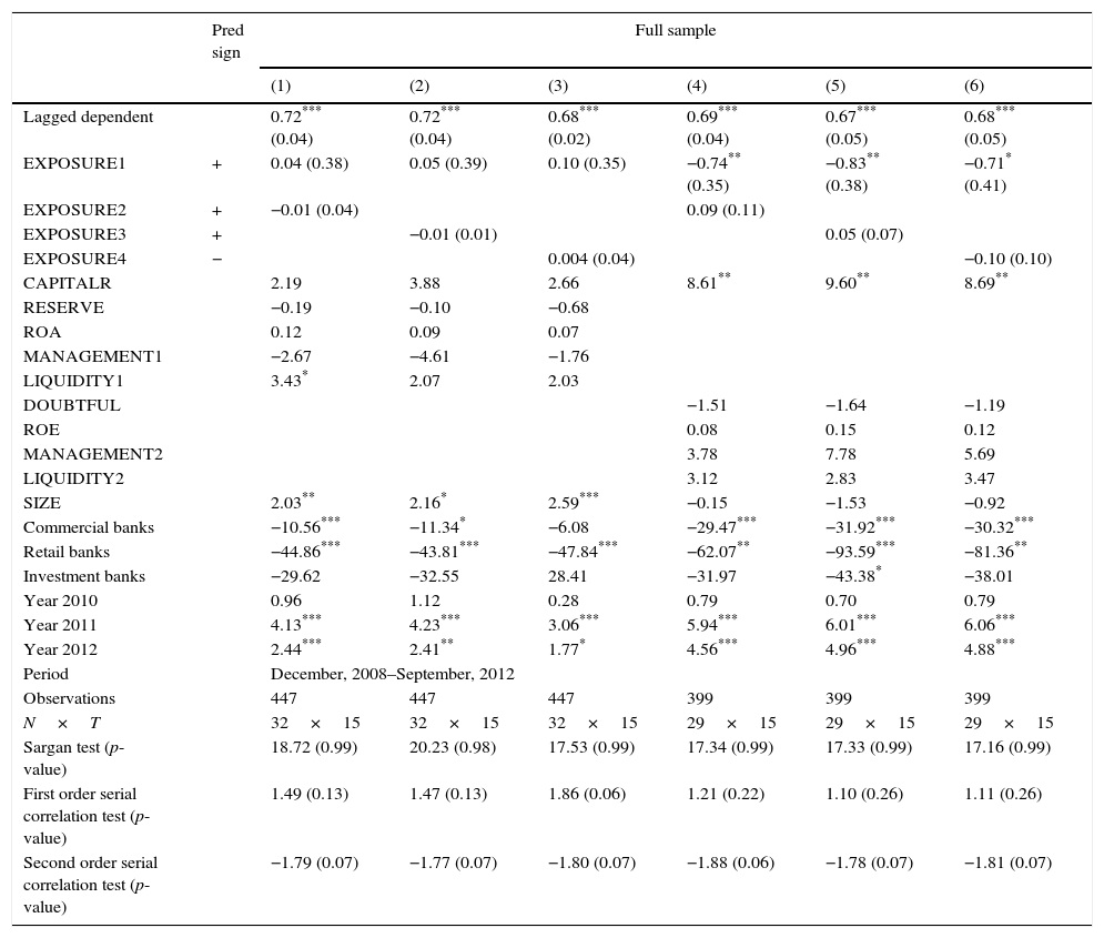
Table 4 summarizes the main results when the measure of bank risk is Z-SCORE. In columns, there are results of the regressions using the full sample with combinations of the explanatory variables (consequently, they check robustness by replacement). The explanatory variables are in rows and empty cells indicate that the variable was dropped because of collinearity.

Table 4.

Z-SCORE – exposure nexus.

	Pred sign	Full sample
		(1)	(2)	(3)	(4)	(5)	(6)
Lagged dependent		0.72^*** (0.04)	0.72^*** (0.04)	0.68^*** (0.02)	0.69^*** (0.04)	0.67^*** (0.05)	0.68^*** (0.05)
EXPOSURE1	+	0.04 (0.38)	0.05 (0.39)	0.10 (0.35)	−0.74^** (0.35)	−0.83^** (0.38)	−0.71^* (0.41)
EXPOSURE2	+	−0.01 (0.04)			0.09 (0.11)
EXPOSURE3	+		−0.01 (0.01)			0.05 (0.07)
EXPOSURE4	−			0.004 (0.04)			−0.10 (0.10)
CAPITALR		2.19	3.88	2.66	8.61^**	9.60^**	8.69^**
RESERVE		−0.19	−0.10	−0.68
ROA		0.12	0.09	0.07
MANAGEMENT1		−2.67	−4.61	−1.76
LIQUIDITY1		3.43^*	2.07	2.03
DOUBTFUL					−1.51	−1.64	−1.19
ROE					0.08	0.15	0.12
MANAGEMENT2					3.78	7.78	5.69
LIQUIDITY2					3.12	2.83	3.47
SIZE		2.03^**	2.16^*	2.59^***	−0.15	−1.53	−0.92
Commercial banks		−10.56^***	−11.34^*	−6.08	−29.47^***	−31.92^***	−30.32^***
Retail banks		−44.86^***	−43.81^***	−47.84^***	−62.07^**	−93.59^***	−81.36^**
Investment banks		−29.62	−32.55	28.41	−31.97	−43.38^*	−38.01
Year 2010		0.96	1.12	0.28	0.79	0.70	0.79
Year 2011		4.13^***	4.23^***	3.06^***	5.94^***	6.01^***	6.06^***
Year 2012		2.44^***	2.41^**	1.77^*	4.56^***	4.96^***	4.88^***
Period		December, 2008–September, 2012
Observations		447	447	447	399	399	399
N × T		32 × 15	32 × 15	32 × 15	29 × 15	29 × 15	29 × 15
Sargan test (p-value)		18.72 (0.99)	20.23 (0.98)	17.53 (0.99)	17.34 (0.99)	17.33 (0.99)	17.16 (0.99)
First order serial correlation test (p-value)		1.49 (0.13)	1.47 (0.13)	1.86 (0.06)	1.21 (0.22)	1.10 (0.26)	1.11 (0.26)
Second order serial correlation test (p-value)		−1.79 (0.07)	−1.77 (0.07)	−1.80 (0.07)	−1.88 (0.06)	−1.78 (0.07)	−1.81 (0.07)

	Pred sign	Full sample (including investment banks)
		(7)	(8)	(9)	(10)	(11)	(12)
Lagged dependent		0.73^*** (0.02)	0.73^*** (0.02)	0.73^*** (0.02)	0.71^*** (0.03)	0.69^*** (0.02)	0.71^*** (0.03)
EXPOSURE1	+	−0.06 (0.14)	−0.02 (0.14)	−0.01 (0.14)	−0.55^* (0.29)	−0.40^* (0.21)	−0.43 (0.30)
EXPOSURE2	+	0.05^*** (0.01)			0.13^** (0.06)
EXPOSURE3	+		0.01 (0.01)			0.08^** (0.04)
EXPOSURE4	−			−0.05^*** (0.01)			−0.12^* (0.06)
CAPITALR		3.14	3.02	3.14	5.41	8.01^***	5.42
RESERVE		X	X	X	X	X	X
ROA		0.02	−0.0005	0.02
MANAGEMENT1		−7.43^***	−7.62^***	−7.43^***
LIQUIDITY1		1.32^***	1.42^***	1.32^***
DOUBTFUL		X	X	X	X	X	X
ROE					−0.04	−0.09	−0.04
MANAGEMENT2					−3.59	−6.11	−3.48
LIQUIDITY2					1.23^**	1.41^**	1.18^**
SIZE		3.24^***	3.21^***	3.24^***	3.21	3.73^***	3.19
Commercial banks		−27.25^***	−27.17^***	−27.25^***	−18.76^**	−17.47^**	−18.78^**
Retail banks		−38.99^***	−38.61^***	−38.99^***	−59.97^*	−54.60^*	−60.23^*
Investment banks		−13.90	−13.56	−13.90	−10.44	−14.82	−10.43
Year 2010		0.17	0.22	0.17	0.18	0.15	0.20
Year 2011		2.30^***	2.29^***	2.30^***	4.73^***	4.79^***	4.74^***
Year 2012		1.15^*	1.15^*	1.15^*	3.08^***	2.98^***	3.07^***
Period		December, 2008–September, 2012
Observations		546	542	546	457	456	457
N × T		37 × 15	37 × 15	37 × 15	33 × 15	33 × 15	33 × 15
Sargan test (p-value)		23.37 (0.96)	22.71 (0.96)	23.37 (0.96)	20.07 (0.98)	19.84 (0.99)	20.05 (0.98)
First order serial correlation test (p-value)		1.37 (0.16)	1.36 (0.17)	1.37 (0.16)	1.28 (0.19)	1.35 (0.17)	1304 (0.19)
Second order serial correlation test (p-value)		−1.70 (0.08)	−1.71 (0.08)	−1.70 (0.08)	−1.84 (0.06)	−1.74 (0.08)	−1.84 (0.06)

X: Variable excluded to allow the inclusion of more investment banks in the sample.

Regressions are estimated using the dynamic SYS GMM estimator (Blundell and Bond, 1998).

In parentheses are standard errors (only for the key explanatory variables and the dependent as regressor).

*

indicates statistical significance at the 10% level.

**

indicates statistical significance at the 5% level.

***

indicates statistical significance at the 1% level.

It is noteworthy that the dynamic panel is justified because the dependent variables as regressors show statistically significant coefficients at the 1% level. All reported estimations pass both the Sargan and the first order serial correlation tests at conventional significance levels, although the second order serial correlation test shows some problems.

In the columns (1)–(6), only the indicator of exposure as lender (EXPOSURE1) shows some statistically significant coefficients with negative signs. Hence, banks with more exposure to the interbank market as lenders present higher levels of risk. Nevertheless, this result must be treated with caution because other regressions, with other control variables (see columns 1–3), do not support this finding. Moreover, as described above, in the section on descriptive statistics, the largest banks are net lenders, and the individual analysis of the G7 banks does not show evidence in favor of this finding, as will be discussed below.

The other measures of exposure to the interbank market (as borrower) do not have statistical significance (see columns 1–6). Thus, the exposure to the interbank market as borrower does not affect the levels of risk-taking, and these first findings do not support the peer monitoring hypothesis. Note that a few control variables, in specific the CAMEL indicators, enter significantly in the regressions.

The number of banks in each regression diminishes because of data limitations on investment banks (see row N × T in Table 4). The information on the variables RESERVE and DOUBTFUL is available only for two investment banks. As a result, the majority of investment banks are not included in the regressions (1)–(6). I removed RESERVE and DOUBTFUL as control variables, to include these banks in the analysis, and the new results are reported in the columns (7)–(12) in Table 4. Now, most of the exposure variables (EXPOSURE2–4) have statistically significant coefficients with the predicted sign, in favor of the peer monitoring hypothesis. Moreover, the control variables LIQUIDITY and MANAGEMENT enter significantly in the majority of the regressions.

It is interesting to note that in most of the regressions bank size has statistically significant coefficients with a positive sign, so larger banks show lower levels of risk. The dummies for year 2011 and 2012 have positive and significant coefficients in all regressions, as it was expected, because Z-SCORE has a positive trend in the last years.

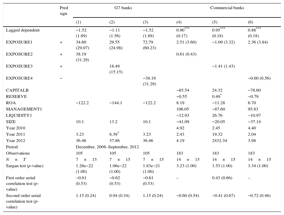
The dummies for commercial and retail banks enter with negative and statistically significant coefficients. Subsequently, these types of banks have lower levels of Z-SCORE (they are riskier) in comparison with the G7 banks (the reference group). Besides, this indicates that the regression results depend on types of banks. Accordingly, I replicated the regressions by subsamples of banks. Table 5 shows the major findings. The problem of multicollinearity among control variables is higher, but different combinations of control variables showed similar results to those reported in Table 5.⁵

Table 5.

Z-SCORE – exposure nexus by subsamples of banks.

	Pred sign	G7 banks			Commercial banks
		(1)	(2)	(3)	(4)	(5)	(6)
Lagged dependent		−1.52 (1.89)	−1.11 (1.56)	−1.52 (1.89)	0.90^*** (0.17)	0.95^*** (0.18)	0.88^*** (0.18)
EXPOSURE1	+	34.60 (29.07)	29.55 (24.98)	72.79 (60.23)	2.51 (3.60)	−1.09 (3.32)	2.36 (3.84)
EXPOSURE2	+	38.19 (31.29)			0.61 (0.43)
EXPOSURE3	+		18.49 (15.15)			−1.41 (1.43)
EXPOSURE4	−			−38.19 (31.29)			−0.60 (0.56)
CAPITALR					−85.54	24.32	−78.60
RESERVE					−0.55	0.49^*	−0.79
ROA		−122.2	−144.1	−122.2	8.19	−11.28	6.70
MANAGEMENT1					106.05	−87.60	95.83
LIQUIDITY1					−12.93	26.76	−10.97
SIZE		10.1	13.2	10.1	−41.09	−20.05	−37.14
Year 2010					4.92	2.45	4.40
Year 2011		3.23	8.39^*	3.23	2.43	19.32	2.04
Year 2012		36.46	37.86	36.46	4.19	2432.34	3.98
Period		December, 2008–September, 2012
Observations		105	105	105	183	183	183
N × T		7 × 15	7 × 15	7 × 15	14 × 15	14 × 15	14 × 15
Sargan test (p-value)		1.26e−22 (1.00)	1.06e−22 (1.00)	1.83e−21 (1.00)	3.23 (1.00)	1.53 (1.00)	3.34 (1.00)
First order serial correlation test (p-value)		−0.61 (0.53)	−0.62 (0.53)	−0.61 (0.53)	–	0.43 (0.66)	–
Second order serial correlation test (p-value)		1.15 (0.24)	0.94 (0.34)	1.15 (0.24)	−0.60 (0.54)	−0.41 (0.67)	−0.72 (0.46)

	Pred sign	Retail banks			Investment banks
		(7)	(8)	(9)	(10)	(11)	(12)
Lagged dependent		1.45 (0.92)	1.39^* (0.74)	1.46^* (0.89)	−0.11 (0.71)	0.17 (2.18)	−0.11 (0.71)
EXPOSURE1	+	1.86 (7.09)	−0.14 (13.25)	2.40 (5.30)	−0.51 (5.02)	−3.75 (50.86)	0.10 (3.77)
EXPOSURE2	+	0.16 (0.12)			0.61 (1.92)
EXPOSURE3	+		0.12 (0.16)			−0.81^* (0.47)
EXPOSURE4	−			−0.14 (0.36)			−0.61 (1.92)
CAPITALR		1.84	−0.21	1.80
RESERVE			−23.44
ROA		0.17	8.07	0.16	10.06	−6.74	10.06
MANAGEMENT1		−17.41	25.38	−18.00
LIQUIDITY1		2.09	−0.21	2.11	5.83	−3.92	5.83^*
SIZE		3.09	−23.44	3.34	−3.55	−27.55	−3.55
Year 2010
Year 2011
Year 2012		−5.47	−3.42	−5.53	3.82	−878.47^*	3.82
Period		December, 2008–September, 2012
Observations		129	129	129	104	100	104
N × T		9 × 15	9 × 15	9 × 15	7 × 15	7 × 15	7 × 15
Sargan test (p-value)		6.11e22 (1.00)	9.73e25 (1.00)	4.20e22 (1.00)	6.64e22 (1.00)	1.08e20 (1.00)	2.82e22 (1.00)
First order serial correlation test (p-value)		0.06 (0.95)	−0.08 (0.93)	0.06 (0.95)	−0.07 (0.94)	0.46 (0.64)	−0.07 (0.94)
Second order serial correlation test (p-value)		−0.01 (0.98)	0.34 (0.72)	−0.04 (0.96)	0.20 (0.83)	0.40 (0.68)	0.20 (0.83)

Regressions are estimated using the dynamic SYS GMM estimator (Blundell and Bond, 1998).

In parentheses are standard errors (only for the key explanatory variables and the dependent as regressor).

*

indicates statistical significance at the 10% level.

** indicates statistical significance at the 5% level.

***

indicates statistical significance at the 1% level.

The regressions by subsamples of banks do not present evidence in favor of the peer monitoring hypothesis. All reported estimations pass the Sargan and the first and second order serial correlation tests, yet the model lost meaning for the G7 banks and investment banks, where practically nothing is explaining the levels of Z-SCORE. In the case of commercial and retail banks, only the dependent variable as regressor has statistical significance.

Consequently, the previous findings about the presence of market discipline in the Mexican interbank market are not robust. The statistical significance of the bank risk-exposure nexus depends on the inclusion of investment banks. Without these banks, as reference, the rest of banks do not show evidence in favor of the peer monitoring hypothesis. Furthermore, the exposure to the interbank market by types of banks (subsamples) does not present a significant relationship with Z-SCORE (bank risk).

These findings also imply that the monitoring activities, if they exist, works from one region (market share or sector) to another, as described by Allen and Gale (2000), probably from the G7 (net lenders) to investment banks. I do not find evidence for peer monitoring from one bank to other bank inside of their banking groups. However, it is worth noting that the results do not indicate that the exposure to the interbank market increases the bank risk.

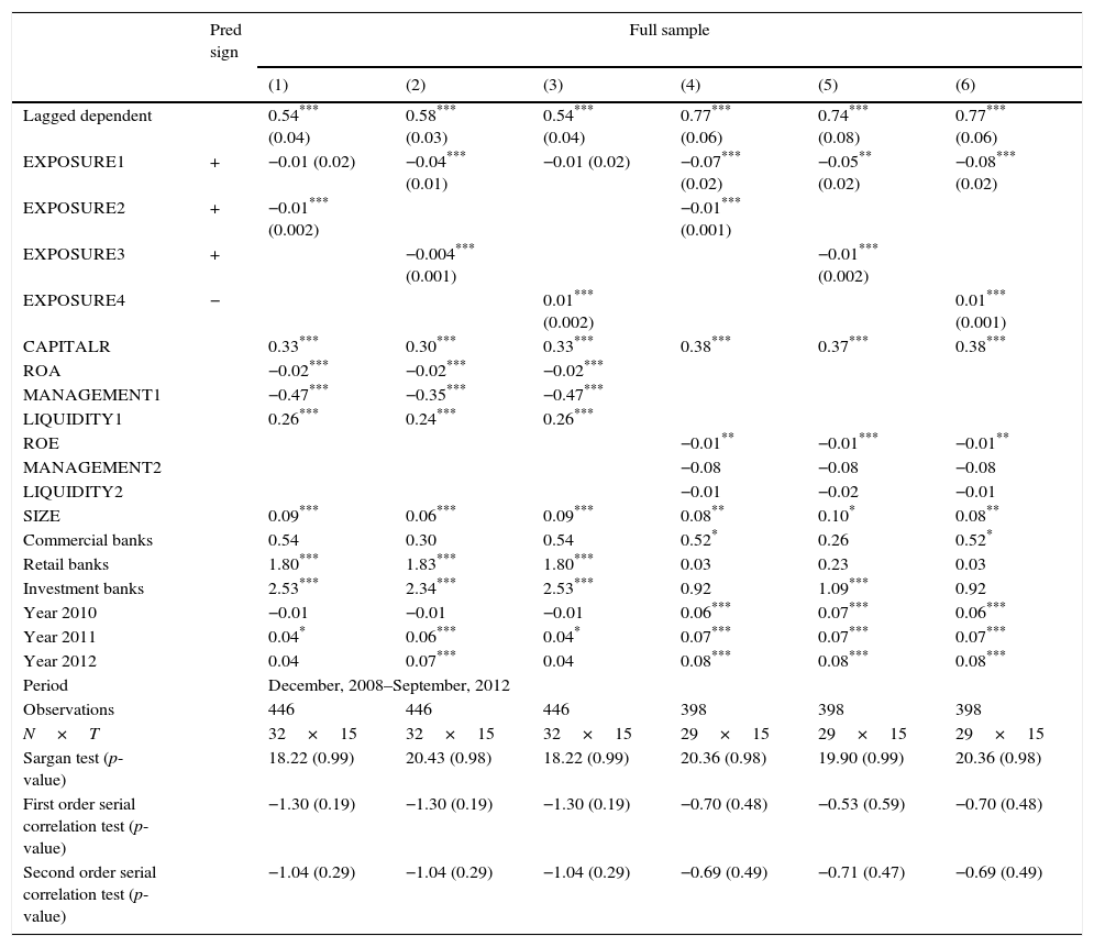
Table 6 summarizes the main results when the bank risk is approached with RESERVE. In columns, there are results of the regressions using the full sample and subsamples, but I excluded the subsample of investment banks because of data limitations (RESERVE is available only for two investment banks). All reported estimations pass both the Sargan and the first and second order serial correlation tests.

Table 6.

RESERVE – exposure nexus.

	Pred sign	Full sample
		(1)	(2)	(3)	(4)	(5)	(6)
Lagged dependent		0.54^*** (0.04)	0.58^*** (0.03)	0.54^*** (0.04)	0.77^*** (0.06)	0.74^*** (0.08)	0.77^*** (0.06)
EXPOSURE1	+	−0.01 (0.02)	−0.04^*** (0.01)	−0.01 (0.02)	−0.07^*** (0.02)	−0.05^** (0.02)	−0.08^*** (0.02)
EXPOSURE2	+	−0.01^*** (0.002)			−0.01^*** (0.001)
EXPOSURE3	+		−0.004^*** (0.001)			−0.01^*** (0.002)
EXPOSURE4	−			0.01^*** (0.002)			0.01^*** (0.001)
CAPITALR		0.33^***	0.30^***	0.33^***	0.38^***	0.37^***	0.38^***
ROA		−0.02^***	−0.02^***	−0.02^***
MANAGEMENT1		−0.47^***	−0.35^***	−0.47^***
LIQUIDITY1		0.26^***	0.24^***	0.26^***
ROE					−0.01^**	−0.01^***	−0.01^**
MANAGEMENT2					−0.08	−0.08	−0.08
LIQUIDITY2					−0.01	−0.02	−0.01
SIZE		0.09^***	0.06^***	0.09^***	0.08^**	0.10^*	0.08^**
Commercial banks		0.54	0.30	0.54	0.52^*	0.26	0.52^*
Retail banks		1.80^***	1.83^***	1.80^***	0.03	0.23	0.03
Investment banks		2.53^***	2.34^***	2.53^***	0.92	1.09^***	0.92
Year 2010		−0.01	−0.01	−0.01	0.06^***	0.07^***	0.06^***
Year 2011		0.04^*	0.06^***	0.04^*	0.07^***	0.07^***	0.07^***
Year 2012		0.04	0.07^***	0.04	0.08^***	0.08^***	0.08^***
Period		December, 2008–September, 2012
Observations		446	446	446	398	398	398
N × T		32 × 15	32 × 15	32 × 15	29 × 15	29 × 15	29 × 15
Sargan test (p-value)		18.22 (0.99)	20.43 (0.98)	18.22 (0.99)	20.36 (0.98)	19.90 (0.99)	20.36 (0.98)
First order serial correlation test (p-value)		−1.30 (0.19)	−1.30 (0.19)	−1.30 (0.19)	−0.70 (0.48)	−0.53 (0.59)	−0.70 (0.48)
Second order serial correlation test (p-value)		−1.04 (0.29)	−1.04 (0.29)	−1.04 (0.29)	−0.69 (0.49)	−0.71 (0.47)	−0.69 (0.49)

	Pred sign	G7 banks			Commercial banks			Retail banks
		(7)	(8)	(9)	(10)	(11)	(12)	(13)	(14)	(15)
Lagged dependent		−1.74 (1.63)	0.63 (3.47)	1.89 (4.84)	−2.91^* (1.45)	0.14 (0.34)	−2.91^** (1.45)	−0.61 (0.70)	−0.46 (0.81)	−0.56 (0.67)
EXPOSURE1	+	0.05 (0.07)	−0.10 (0.75)	−0.22 (0.87)	0.13 (0.10)	−0.01 (0.04)	0.13 (0.10)	0.36 (0.69)	6.97 (8.43)	0.38 (0.70)
EXPOSURE2	+	−0.19 (0.20)			−0.004 (0.01)			0.02 (0.03)
EXPOSURE3	+		0.09 (0.23)			−0.01 (0.01)			0.06 (0.07)
EXPOSURE4	−			−0.01 (0.11)			0.004 (0.01)			−0.03 (0.03)
CAPITALR		0.84^**			−1.42	1.52	−1.42	1.64	19.90	1.62
ROA		−0.23	−1.12	−2.20	−0.44^*	−0.21	−0.44^*	−0.003	−0.81	−0.003
MANAGEMENT1					−5.16	0.48	−5.16	−0.35	−11.48	−0.36
LIQUIDITY1		0.64	−1.02	−3.14	−1.22^*	0.82^*	−1.22^*	0.44	5.17	0.44
ROE
MANAGEMENT2
LIQUIDITY2
SIZE				−6.39	−1.58	1.70^*	−1.58	0.93	12.02	0.97
Commercial banks
Retail banks
Investment banks
Year 2010					−0.13	−0.07	−0.13
Year 2011			0.07		0.27	−0.26	0.27
Year 2012		−7.16	7.66	−0.10	0.57	−0.31	0.57	0.08	0.01	0.08
Period		December, 2008–September, 2012
Observations		105	105	105	181	181	181	130	130	130
N × T		7 × 15	7 × 15	7 × 15	14 × 15	14 × 15	14 × 15	9 × 15	9 × 15	9 × 15
Sargan test (p-value)		7.69e26 (1.00)	1.50e24 (1.00)	8.60e22 (1.00)	2.90 (1.00)	3.18 (1.00)	2.90 (1.00)	1.85e24 (1.00)	4.84e21 (1.00)	4.42e25 (1.00)
First order serial correlation test (p-value)		0.59 (0.54)	−0.16 (0.87)	−0.39 (0.69)	0.52 (0.60)	−0.83 (0.40)	0.52 (0.60)	0.55 (0.57)	−0.08 (0.93)	0.52 (0.59)
Second order serial correlation test (p-value)		−0.65 (0.51)	–	−0.39 (0.69)	0.72 (0.46)	−0.17 (0.86)	0.72 (0.46)	−0.43 (0.66)	−0.53 (0.59)	−0.42 (0.67)

Regressions are estimated using the dynamic SYS GMM estimator (Blundell and Bond, 1998).

In parentheses are standard errors (only for the key explanatory variables and the dependent as regressor).

*

indicates statistical significance at the 10% level.

**

indicates statistical significance at the 5% level.

***

indicates statistical significance at the 1% level.

Specifically, the dynamic model is justified for the full sample where the dependent variable as regressor enters with statistically significant coefficients at the 1% level (see columns 1–6 in Table 6). In this case, the measures of exposure to the interbank market (as lender or borrower), in general, have statistical significance, yet with the opposite sign. Banks with higher exposure to the interbank market, especially as borrower, present lower levels of RESERVE, so they are riskier. This is evidence against the peer monitoring hypothesis, and in favor of the contagion hypothesis.

The majority of the control variables enter in the model with statistically significant coefficients, I will not comment further on that to save space. Nevertheless, note that the dummies for types of banks show some significant coefficients with positive signs, suggesting a bias by subsamples of banks, as in the previous model.

Columns (7)–(15) in Table 6 show the estimations by subsamples. For a second time, the EXPOSURE variables do not present significance in any case. This result may imply that the channel of contagion, if it appears, is from one region to another, it is not from one bank to another. Anyway, the peer monitoring is absent.

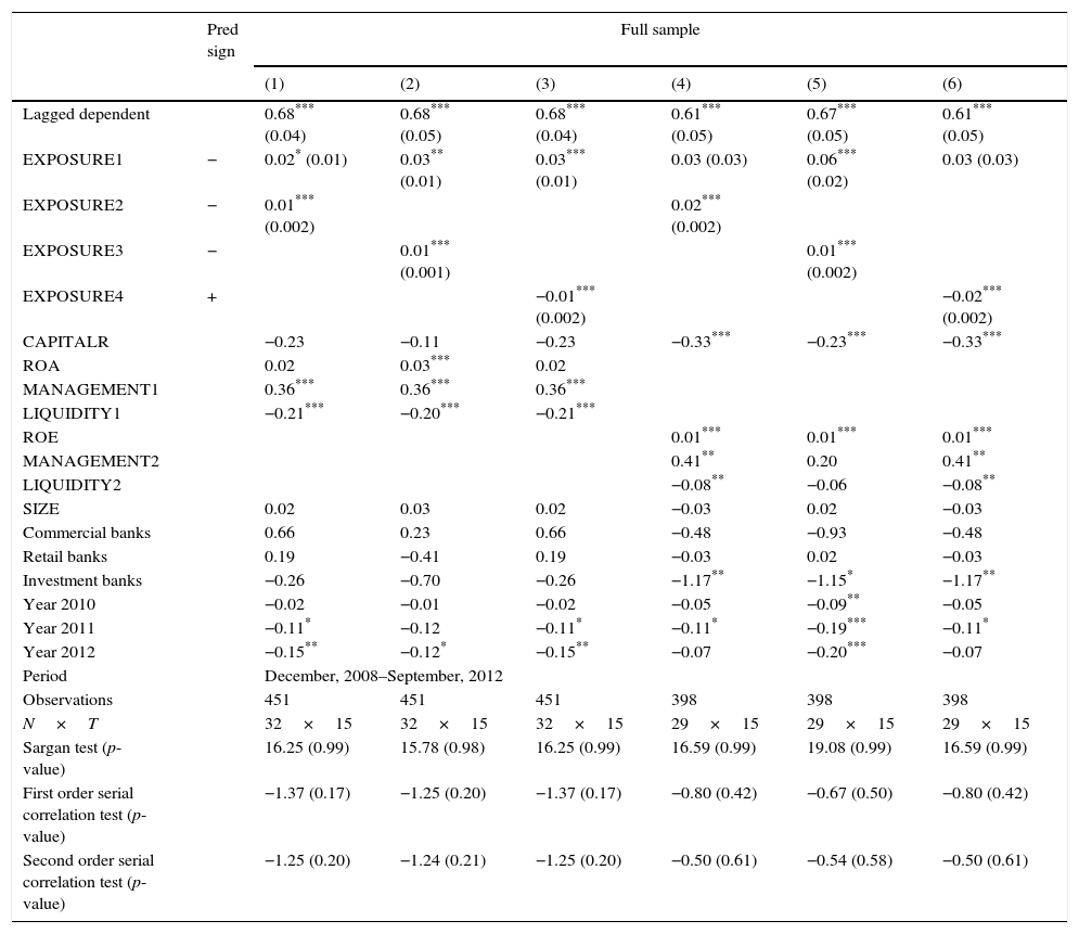
Table 7 summarizes the main results when the measure of bank risk is DOUBTFUL. All reported estimations pass both the Sargan and the first and second order serial correlation tests. I expect an inverse relationship with exposure to the interbank market because higher values of DOUBTFUL indicate riskier banks.

Table 7.

DOUBTFUL – exposure nexus.

	Pred sign	Full sample
		(1)	(2)	(3)	(4)	(5)	(6)
Lagged dependent		0.68^*** (0.04)	0.68^*** (0.05)	0.68^*** (0.04)	0.61^*** (0.05)	0.67^*** (0.05)	0.61^*** (0.05)
EXPOSURE1	−	0.02^* (0.01)	0.03^** (0.01)	0.03^*** (0.01)	0.03 (0.03)	0.06^*** (0.02)	0.03 (0.03)
EXPOSURE2	−	0.01^*** (0.002)			0.02^*** (0.002)
EXPOSURE3	−		0.01^*** (0.001)			0.01^*** (0.002)
EXPOSURE4	+			−0.01^*** (0.002)			−0.02^*** (0.002)
CAPITALR		−0.23	−0.11	−0.23	−0.33^***	−0.23^***	−0.33^***
ROA		0.02	0.03^***	0.02
MANAGEMENT1		0.36^***	0.36^***	0.36^***
LIQUIDITY1		−0.21^***	−0.20^***	−0.21^***
ROE					0.01^***	0.01^***	0.01^***
MANAGEMENT2					0.41^**	0.20	0.41^**
LIQUIDITY2					−0.08^**	−0.06	−0.08^**
SIZE		0.02	0.03	0.02	−0.03	0.02	−0.03
Commercial banks		0.66	0.23	0.66	−0.48	−0.93	−0.48
Retail banks		0.19	−0.41	0.19	−0.03	0.02	−0.03
Investment banks		−0.26	−0.70	−0.26	−1.17^**	−1.15^*	−1.17^**
Year 2010		−0.02	−0.01	−0.02	−0.05	−0.09^**	−0.05
Year 2011		−0.11^*	−0.12	−0.11^*	−0.11^*	−0.19^***	−0.11^*
Year 2012		−0.15^**	−0.12^*	−0.15^**	−0.07	−0.20^***	−0.07
Period		December, 2008–September, 2012
Observations		451	451	451	398	398	398
N × T		32 × 15	32 × 15	32 × 15	29 × 15	29 × 15	29 × 15
Sargan test (p-value)		16.25 (0.99)	15.78 (0.98)	16.25 (0.99)	16.59 (0.99)	19.08 (0.99)	16.59 (0.99)
First order serial correlation test (p-value)		−1.37 (0.17)	−1.25 (0.20)	−1.37 (0.17)	−0.80 (0.42)	−0.67 (0.50)	−0.80 (0.42)
Second order serial correlation test (p-value)		−1.25 (0.20)	−1.24 (0.21)	−1.25 (0.20)	−0.50 (0.61)	−0.54 (0.58)	−0.50 (0.61)

	Pred sign	G7 banks			Commercial banks			Retail banks
		(7)	(8)	(9)	(10)	(11)	(12)	(13)	(14)	(15)
Lagged dependent		1.16 (1.57)	0.60 (1.30)	1.16 (1.57)	0.57 (0.47)	1.11 (0.78)	0.57 (0.47)	1.53 (2.30)	−1.37 (2.54)	2.99 (6.52)
EXPOSURE1	−	0.03 (0.11)	−0.01 (0.06)	0.12 (0.60)	−0.06 (0.19)	−0.05 (0.23)	−0.04 (0.19)	−0.03 (0.06)	−0.12 (0.09)	0.18 (0.64)
EXPOSURE2	−	0.10 (0.50)			0.02 (0.02)			0.02 (0.04)
EXPOSURE3	−		−0.03 (0.03)			0.03 (0.02)			0.01 (0.02)
EXPOSURE4	+			−0.10 (0.50)			−0.02 (0.02)			−0.07 (0.19)
CAPITALR					0.38	−0.59	0.38	3.25	−3.80	13.02
ROA		0.59	−0.05	0.59	−0.20	0.10	−0.20	0.03	−0.11	0.09
MANAGEMENT1					1.39	4.92	1.39	2.77	0.73	2.35
LIQUIDITY1		2.58	0.89	2.58	−0.24	−0.17	−0.24	−0.11	0.87	−0.23
ROE
MANAGEMENT2
LIQUIDITY2
SIZE					−0.33	−0.63	−0.33	2.07	1.67	2.76
Commercial banks
Retail banks
Investment banks
Year 2010					0.02	0.29	0.02
Year 2011		−13.54	3.58	−13.54	−0.48	−0.23	−0.48
Year 2012		−13.23	3.66	−13.23	−0.48	−0.16	−0.48	0.01	2.63	−0.10
Period		December, 2008–September, 2012
Observations		105	105	105	186	186	186	130	130	130
N × T		7 × 15	7 × 15	7 × 15	14 × 15	14 × 15	14 × 15	9 × 15	9 × 15	9 × 15
Sargan test (p-value)		3.51e20 (1.00)	4.92e22 (1.00)	9.68e21 (1.00)	3.16 (1.00)	3.71 (1.00)	3.16 (1.00)	3.47e24 (1.00)	5.22e22 (1.00)	2.34e22 (1.00)
First order serial correlation test (p-value)		−0.09 (0.92)	−0.25 (0.79)	−0.09 (0.92)	−0.43 (0.66)	−0.17 (0.86)	−0.43 (0.66)	0.73 (0.46)	0.57 (0563)	0.41 (0.67)
Second order serial correlation test (p-value)		0.27 (0.78)	−0.21 (0.82)	0.27 (0.78)	−0.21 (0.82)	−0.50 (0.61)	−0.21 (0.82)	0.77 (0.43)	−0.13 (0.89)	0.36 (0.71)

Regressions are estimated using the dynamic SYS GMM estimator (Blundell and Bond, 1998).

In parentheses are standard errors (only for the key explanatory variables and the dependent as regressor).

*

indicates statistical significance at the 10% level.

**

indicates statistical significance at the 5% level.

***

indicates statistical significance at the 1% level.

The results are similar to the RESERVE case. The full sample again shows evidence in opposition to the peer monitoring hypothesis, and in favor of the contagion hypothesis. The coefficients of the EXPOSURE variables, especially as borrower, present statistically significant coefficients with the opposite sign, so banks with larger exposure to the interbank market are riskier. Once more, the regressions by subsamples of banks do not show any significance, and the subsample of investment banks was excluded because of data limitations (DOUBTFUL is available only for two investment banks).

Summarizing, the bank risk-exposure nexus in the Mexican interbank market rejects the peer monitoring hypothesis. With three different measures of bank risk the regression analysis indirectly suggest evidence in favor of the contagion hypothesis, because banks with higher exposure to the interbank market, especially as borrower, present higher levels of risk (lower levels of RESERVE and higher levels of DOUBTFUL). It is important to note that, in general, the regressions by subsamples of banks do not show statistical significance, and this finding can be interpreted as connections from one banking sector to another. These results are robust to different combinations of explanatory and control variables. In particular, the regressions with EXPOSURE2 and EXPOSURE4 show very similar coefficients for the independent variables.

Although, there is no reason to assume that the variables have unit roots and are thus non-stationary, as additional robustness checks, I also estimated the equation 2 using the DIF GMM method, which has a better control on non-stationary variables because the model is in first differences. The results are very similar to those reported in Tables 3–6. In addition, I replicated the regressions using as independent variable the ratio of the indicator of exposure to the corresponding indicator of bank risk (the ratio of exposure to risk-taking). This strategy can reduce the simultaneity problem; however, the regressions presented autocorrelation concerns, yet the major findings are similar (these results are not reported in tables to conserve space).

5

Conclusions

Theoretically, bankers are well equipped to identify low-quality banks, and banks with larger exposure to the interbank market should show lower bank risk. Previous empirical studies found evidence in favor of this bank risk-exposure nexus (Dinger and Von Hagen, 2009; Distinguin et al., 2013). Nevertheless, the interbank market also is a channel for contagion.

In this paper I studied the Mexican case over the period from December 2008 to September 2012, using regression analysis (dynamic panel models) and a large range of dependent and explanatory variables to check robustness, I did not find evidence for market discipline. On the contrary, some findings indirectly suggest that the interbank market can facilitate the contagion, similar results were found in the Dutch case (Liedorp et al., 2010).

The empirical tests on the bank risk-exposure nexus demonstrate that Mexican banks with larger exposure to the interbank market show larger loan losses. In other words, lower levels of reserve for loan losses (RESERVE) and higher levels of nonperforming loans (DOUBTFUL), indicating a higher probability of bank failure.

When the measure of bank risk is Z-SCORE the findings show mixed evidence. Regressions including investment banks show evidence in favor of the market discipline hypothesis where banks with higher exposure to the interbank market present lower bank risk (higher values of Z-SCORE). However, the regressions do not show evidence for market discipline by peer monitoring without the inclusion of investment banks. Moreover, the regressions by subsamples of banks (G7, commercial, retail and investment banks) lack in statistical significance, which indicates that interbank transactions might principally be from one banking sector to another. Therefore, these transactions are not from one bank to other bank, and the largest banks (G7) function as net lenders.

These findings have several implications for Mexican policymakers, who cannot appeal to the market to regulate the risky behavior of banks in interbank transactions. Rochet and Tirole (1996) point out that government intervention can destroy peer monitoring among banks, and Distinguin et al. (2013) empirically found that regulatory discipline weakens market discipline. Therefore, policymakers must develop a regulatory framework with enough accessible information to economic agents, who must feel at risk due to their decisions in the banking market. Probably Mexican bankers, especially the largest banks (G7), which are net lenders, think that the government will take actions in accordance with the understood policies too-big-to-fail and too-interconnected-to-fail.

This study presents data limitations, especially for investment banks. Therefore, future research for Mexico must attempt to investigate market discipline in interbank operations including in the sample more investment banks. Also, further research is required to examine connections among groups of Mexican banks (region by region) to identify channels and probabilities of contagion, that is, to test directly the contagion hypothesis. In addition, classic tests on the mechanisms of market discipline (price, quantity, and maturity) are necessary for a deeper analysis of the peer monitoring hypothesis.

Acknowledgment

The article was prepared within the framework of the Academic Fund Program at the National Research University Higher School of Economics (HSE) in 2015 (grant № 16-01-0008) and supported within the framework of a subsidy granted to the HSE by the Government of the Russian Federation for the implementation of the Global Competitiveness Program.