


This paper proposes an ICAPM in which the risk premium embedded in variance swaps is the factor mimicking portfolio for hedging exposure to changes in future investment conditions. Recent empirical evidence shows that the fears by investors to deviations from Normality in the distribution of returns are able to explain time-varying financial and macroeconomic risks in addition to being a determinant of the variance risk premium. Moreover, variance swaps hedges unfavorable changes in the stochastic investment opportunity set, and is not a redundant asset because significantly expands the efficient mean-variance frontier. Thence, we should expect the variance swap risk premium to be priced in the market. We report relatively favorable evidence on the incremental pricing information associated with the variance risk premium, particularly at shorter horizons.
As shown by Carr and Wu (2009), Todorov (2010), and Egloff et al. (2010), the average variance risk premium is negative and sizeable for all available horizons. Since the payoff of a variance swap contract is the difference between the realized variance and the variance swap rate, the observed negative returns for long positions on variance swap contracts for all time horizons suggest that investors are willing to accept negative returns for insuring against future realized variance. Recently, Nieto et al. (2010) use the implications of an asset pricing model proposed by Chabi-Yo (2009) to find evidence that as it is the case with standard indicators of different types of macroeconomic and financial risks, the variance risk premium responds to changes in higher order moments of the conditional distribution of market returns.1 This common dependence suggests that the variance swap may offer hedging against a variety of risks and, consequently, the variance risk premium could be capturing the market willingness to pay for such a hedge.
A natural question then refers to whether the fluctuations in the variance risk premium may act as a sufficient statistic summarizing the information contained in a variety of macroeconomic and financial risk indicators which is relevant for asset valuation. In the continuous-time Intertemporal Asset Pricing Model (ICAPM hereafter) of Merton (1973), the value function depends not only on aggregate wealth, but also on the innovations to some state variables that describe the stochastic behavior of the investment opportunity set. These additional variables may hint at ways to design an appropriate hedge against unfavorable changes in the stochastic investment opportunities and the optimal portfolio should be made up by a combination of the market and the hedging portfolios. In this paper, we employ the payoff of the variance swap as the hedging variable for alternative investment horizons. Therefore, we take the ICAPM as the natural framework to investigate whether the variance risk premium may add information to the return on market wealth as an aggregate risk factor explaining the cross-section of expected returns.2
Specifically, the stochastic discount factor (SDF hereafter) is specified as a power function of the return on the market portfolio, expanded with an exponential function of the excess return of the variance swap contract as hedging variable. We perform several empirical tests of the model that suggest that the variance risk premium contains relevant information that helps pricing average stock returns. The measures of the global fit indicate that the model performs better when it includes the variance risk premium factor than when it only incorporates the market return portfolio. This evidence is generally observed for both the non-linear specification and the beta (linear) specification of the model. Specifically, the comparison between the one-factor model and the two-factor model at the one-month investment horizon reveals that the mean absolute pricing error decreases from 0.343 to 0.288 in the non-linear specification, and that the pseudo cross-sectional R-square used in the estimation increases from 0.278 to 0.412 in the beta specification. Moreover, we also show that, on average, test portfolio betas relative to the variance risk premium factor are strongly negative when we allow for regressions with two regimes based on a market return threshold. The relatively favorable evidence on the variance risk premium being a financial factor that is priced in the market is consistent with the result in Nieto et al. (2010), who show that the variance swap is not being spanned by a set of assets composed of government and corporate bonds and the stock market portfolio.3
The paper is organized as follows. Section 2 briefly describes the variance swap contract and defines the variance risk premium. Section 3 contains a description of the data. The two-factor asset pricing model is presented in Section 4, while Section 5 reports the results of the empirical tests. Section 6 concludes with a summary of our findings.
2Variance swap contracts and the variance risk premiumA variance swap is an over-the-counter financial instrument that pays the difference between a standard estimate of the realized variance of the return on a given asset (a stock market index in this case) and the fixed variance swap rate. More in detail, one leg of the variance swap pays an amount based upon the realized variance of the price changes of the underlying asset. Conventionally, these price changes will be daily log returns, based upon the most commonly used closing price. The other leg of the swap pays a fixed amount, the strike, quoted at the deal's inception. Thus the net payoff to the counterparties is the difference between these two values. It is settled in cash at the expiration of the deal, though some cash payments are likely to be made along the way by one or the other counterpart to maintain an agreed upon margin. The payoff of a variance swap issued at time t and maturing at time t+τ is therefore given by,
where Nvar denotes variance notional, also called variance units, RVt,t+τ is the annualized realized variance over the life of the contract, and SWt,t+τ is the delivery price quoted at time t for the variance of the asset between t and t+τ, also known as the variance swap rate. Hence, profits and losses from a variance swap depend directly on the difference between realized and implied variance.
Since variance swaps cost zero at entry, no arbitrage requires that the variance swap rate must be equal to the risk-neutral expected value of the realized variance. Therefore,
where EtQ(.) is the time-t conditional expectation operator under some risk-neutral measure Q. The variance risk premium at period t is then defined as,where EtP(.) is the time-t conditional expectation operator under the physical probability measure P. If investors price variance risk, the variance swap rate will differ from the expected realized variance under P at the corresponding horizon, the difference being the variance risk premium.3Data and descriptive statistics

In this paper we analyze variance swap contracts on the S&P 500 index. Daily variance swap rates on five different maturities from January 4, 1996 to January 31, 2007 are obtained from Bank of America. We get monthly data by using the quotes on the last day of each month. Our estimation of the realized variance employs intra-daily data observed at 30-min intervals, from 9 a.m. to 3 p.m., on the S&P 500 index returns provided by the Institute of Financial Markets. For each month in our sample, we compute the realized variance for each maturity τ of a variance swap contract (τ=1, 2, 3, 6, and 12 months) using quadratic changes on the value of the S&P 500 index, as given by
where Pt is the level of the index at time t, L is the number of 30-min intervals comprised in the interval (t, t+τ). We work with variance swap rates and realized variances in percent numbers.
For each month t and each maturity τ we compute the log variance risk premium as the logarithm of the ratio between realized variance and the swap rate,
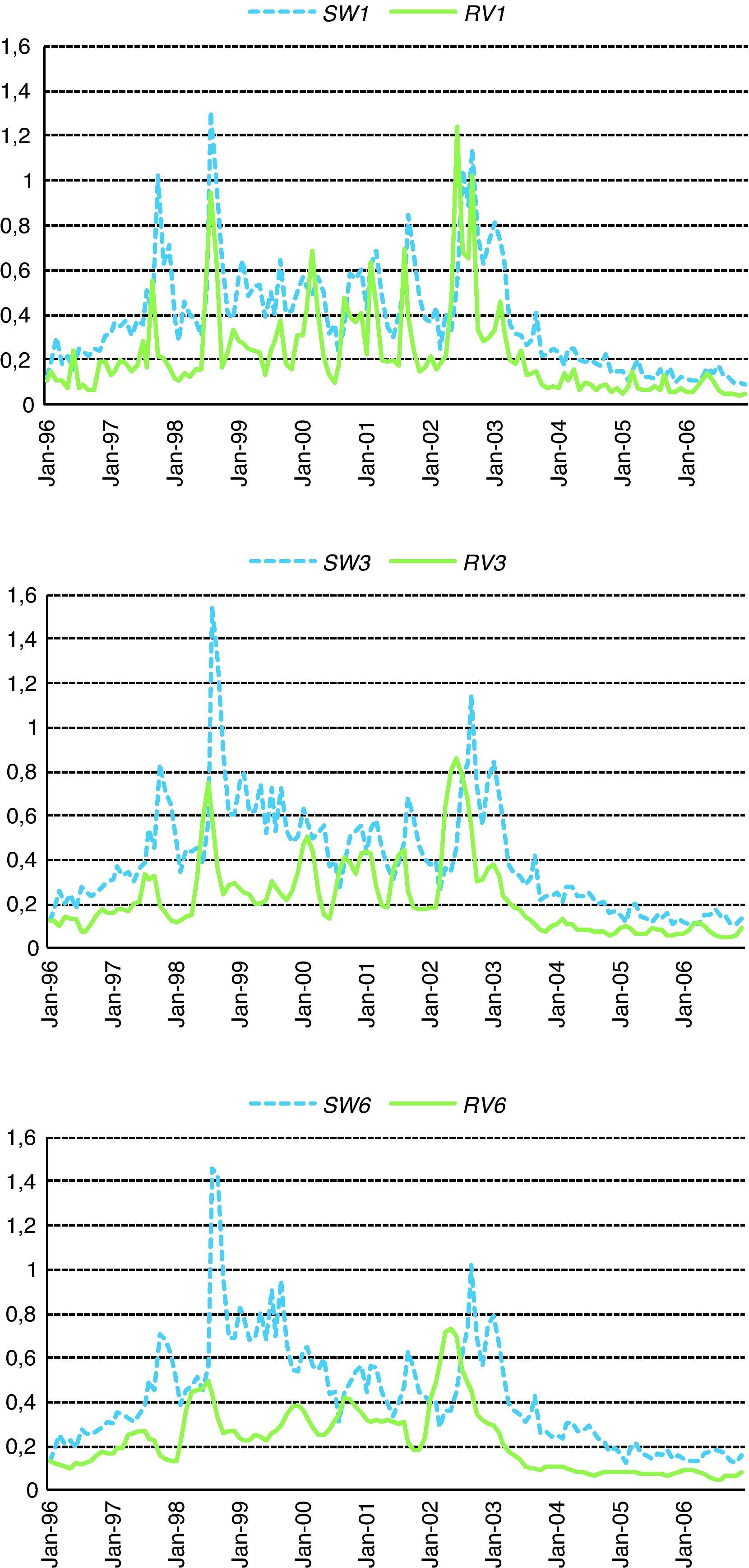
which can be read as the excess rate of return of the variance swap contract. Clearly, VRPtt+τ is known only at time t+τ. Fig. 1 displays variance swap rates and realized variance for 1-, 3- and 6-month maturities. As expected, the swap rate is most often above the level of realized variance, especially for longer maturities. This evidence is similar to that shown by Carr and Wu (2009) for stock market indices and, to a lesser extent, for individual stocks.4 It is clear that investors are willing to accept a significantly negative return to long variance swaps on the S&P index in exchange for being hedged against future unexpected volatility shocks. Therefore, shorting variance swap contracts in the S&P index generates significantly positive average excess returns during our sample period, since the variance risk premium can be seen as the return on holding the variance swap contract.

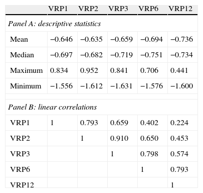
Panel A of Table 1 reports the variance risk premium descriptive statistics for alternative maturities. The variance risk premium is always negative on average, and it becomes more negative with maturity. Panel B of Table 1 reports the correlation coefficients between the variance risk premia at any two different maturities. Correlations between variance risk premia at adjacent maturities are high, debilitating for faraway maturities. The correlation matrix suggests the existence of at least two factors in the structure of variance risk premium.5
Variance risk premia descriptive statistics.
| VRP1 | VRP2 | VRP3 | VRP6 | VRP12 | |
| Panel A: descriptive statistics | |||||
| Mean | −0.646 | −0.635 | −0.659 | −0.694 | −0.736 |
| Median | −0.697 | −0.682 | −0.719 | −0.751 | −0.734 |
| Maximum | 0.834 | 0.952 | 0.841 | 0.706 | 0.441 |
| Minimum | −1.556 | −1.612 | −1.631 | −1.576 | −1.600 |
| Panel B: linear correlations | |||||
| VRP1 | 1 | 0.793 | 0.659 | 0.402 | 0.224 |
| VRP2 | 1 | 0.910 | 0.650 | 0.453 | |
| VRP3 | 1 | 0.798 | 0.574 | ||
| VRP6 | 1 | 0.793 | |||
| VRP12 | 1 | ||||
VRP is the variance risk premium associated with the alternative horizons of the variance swap contract between 1 and 12 months. It is computed as the difference between the ex-post realized variance at the end of the swap contract and the observed variance swap rate.
Monthly data on value-weighted stock market portfolio returns (RW) and the risk-free rate (Rf) are taken from Kenneth French's web page. We also collect the excess returns of 25 size/book-to-market value-weighted portfolios and 17 industry value-weighted portfolios. We compute monthly series of cumulative returns corresponding to the five maturity intervals of the variance swap rates for the market return, the risk-free rate, and the 25 and 17 portfolio returns.
4A two-factor intertemporal asset pricing modelEvidence presented in Nieto et al. (2010) indicates that the variance risk premium is able to anticipate different kinds of risk embedded in traditional state variables, such as the stock market risk, risk of default, illiquidity risk or consumption and employment growth risk. On the other hand, previous empirical literature about the ICAPM shows that innovations to state variables that forecast future investment opportunities seem to be priced by investors.6 It may therefore be the case that the ICAPM holds as a two factor model with the excess return of the variance swap contract as the hedging factor. Bollerslev and Todorov (2010) show that, even though the equity market risk premium and the variance risk premium share similarities in the general dynamic dependencies in jump risk premia, they maintain important differences in the way how they capture the compensations for rare events (tail events).7 Their results imply that any satisfactory model explaining the cross-sectional variation of expected returns should be able to generate a large and time-varying compensation for fears of economic recessions. This is precisely the role that the variance risk premium may be playing in the ICAPM framework.
It is well known that, assuming no arbitrage opportunities, a positive SDF (mt) exists such that,
where Rj,t+1e is the excess return on asset j from t to t+1. The alternative asset pricing models are generated by specifying different SDFs; that is, assuming different preferences for investors or different stochastic processes for asset prices. For example, under the ICAPM, the SDF contains, in addition to the aggregate wealth return, variables that capture time variation in future investment opportunities. Although the model is generally accepted because evidence shows that state variables other than the market index are important for pricing stock returns, the debate about which state variables must enter in the SDF remains open. Therefore, a natural question to ask is whether the information embedded in fluctuations in the variance risk premium may act as a sufficient statistic summarizing relevant information for asset valuation.
To explore this possibility, we use five time horizons corresponding to the five maturities of the swap contracts and data sampled at monthly frequency, to estimate the following ICAPM specification
where RW,t+τ is the gross cumulative return on wealth between t and t+τ, VRPtt+τ is the variance risk premium, i.e., the log-difference between the variance swap rate at month t with maturity on t+τ and the realized variance of the market index between t and t+τ, as defined by expression (5), Rj,t+τe is the excess cumulative return between t and t+τ on asset j, and τ=1, 2, 3, 6 and 12 months.
This SDF specification is consistent with Brennan et al. (2004), and it ensures a positive SDF. These authors argue that if the interest rate and the maximal Sharpe ratio follow a joint Markov process, the investment opportunity set is fully described by their joint dynamics. Accordingly, they propose a three-factor intertemporal model in which the SDF is the product of an exponential function of the innovations of these two variables and a power function of the aggregate wealth return.8
The basic idea behind Eq. (7) relies on focusing on the two key risk premia in financial markets: (i) the equity risk premium for holding the market portfolio, and (ii) the variance risk premium for holding the variance of the market portfolio. It is clear that both risk premia should be correlated. Bollerslev and Todorov (2010) show that roughly 60% of the equity risk premium is due to fears of rare events, while half of the variance risk premium is also due to investor fears. Then, in the empirical estimation of Eq. (7), rather than using directly the variance risk premium, it may be advisable to employ the residuals of a linear projection of the variance risk premium on the market excess portfolio return. Our aim is therefore to test whether the variance risk premium has incremental explanatory power over and above the market portfolio return within an ICAPM framework.
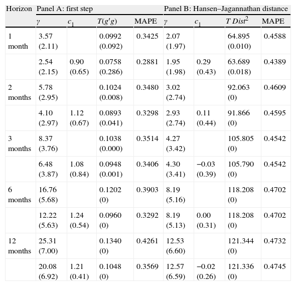
5Asset pricing model performance5.1The non-linear version of the two-factor ICAPMPanel A in Table 2 reports estimates of the coefficients of the iso-elastic SDF, obtained by applying first-stage GMM to Euler Eq. (7), which amounts to minimizing the Euclidean norm of the average vector of pricing errors.9 The test assets are the 25 Fama–French portfolios and 17 industry portfolios. Below each estimate, in parentheses, we report the standard errors that are computed taking into account the fact that pricing errors have different variances and nontrivial covariances. The J-test statistic for overidentifying restrictions, given by T times the sum of the squared pricing errors, T(g′g), is reported in the fourth column, with its p-value in parenthesis. The last column of the table (MAPE) is the mean absolute pricing error across portfolios. We estimate model (7) twice, with and without the exponential factor for the variance risk premium, and for the five time horizons available in our database. The sample frequency is always monthly, from January 2006 to January 2007, which permits the comparison between results across the different horizons and panels of Table 2.
GMM estimation. 25 size/book-to-market portfolios and 17 industry portfolios. Monthly data, January 1996 to January 2007.
| Horizon | Panel A: first step | Panel B: Hansen–Jagannathan distance | ||||||
| γ | c1 | T(g′g) | MAPE | γ | c1 | TDist2 | MAPE | |
| 1 month | 3.57 (2.11) | 0.0992 (0.092) | 0.3425 | 2.07 (1.97) | 64.895 (0.010) | 0.4588 | ||
| 2.54 (2.15) | 0.90 (0.65) | 0.0758 (0.286) | 0.2881 | 1.95 (1.98) | 0.29 (0.43) | 63.689 (0.018) | 0.4389 | |
| 2 months | 5.78 (2.95) | 0.1024 (0.008) | 0.3480 | 3.02 (2.74) | 92.063 (0) | 0.4609 | ||
| 4.10 (2.97) | 1.12 (0.67) | 0.0893 (0.041) | 0.3298 | 2.93 (2.74) | 0.11 (0.44) | 91.866 (0) | 0.4595 | |
| 3 months | 8.37 (3.76) | 0.1038 (0.000) | 0.3514 | 4.27 (3.42) | 105.805 (0) | 0.4542 | ||
| 6.48 (3.87) | 1.08 (0.84) | 0.0948 (0.001) | 0.3406 | 4.30 (3.41) | −0.03 (0.39) | 105.790 (0) | 0.4542 | |
| 6 months | 16.76 (5.68) | 0.1202 (0) | 0.3903 | 8.19 (5.16) | 118.208 (0) | 0.4702 | ||
| 12.22 (5.63) | 1.24 (0.54) | 0.0960 (0) | 0.3292 | 8.19 (5.13) | 0.00 (0.31) | 118.208 (0) | 0.4702 | |
| 12 months | 25.31 (7.00) | 0.1340 (0) | 0.4261 | 12.53 (6.60) | 121.344 (0) | 0.4732 | ||
| 20.08 (6.92) | 1.21 (0.41) | 0.1048 (0) | 0.3569 | 12.57 (6.59) | −0.02 (0.26) | 121.336 (0) | 0.4745 | |
We estimate the standard version and an intertemporal version of the CAPM using the variance risk premium as the hedging factor in the intertemporal specification. The vector of moment conditions is E[((RW,t+τ)−γ exp{c1VRPtt+τ})Rj,t+τe|It+τ−1]=0, where RW is the gross return on wealth, γ is the relative risk aversion coefficient, Rje is the excess return on portfolio j and VRP represents the variance risk premium, computed as the log difference between the realized variance at the end of the swap contract (t+τ) and the variance swap rate at the beginning of the contract (t). We use a linear projection to compute the component of the variance risk premium that is orthogonal to the market return. The estimation is made for different investment horizons (τ), from 1- to 12-months, using always monthly data. Results reported on Panel A refer to the first step GMM estimation while the estimates shown in Panel B have been obtained using the inverse of covariance matrix of the portfolio excess returns as weighting matrix. Columns 2, 3, 6, and 7 contain the estimated coefficients. Associated standard errors are shown below, in brackets. Column 4 provides the value of T times the sum of squared pricing errors. The p-value for the test of overidentifying conditions is shown in brackets, while in Panel B the specification test of the model is performed using the Hansen–Jagannathan distance (column 9). Finally, MAPE indicates the mean absolute pricing error across portfolios, in percentage terms.
When we use the identity matrix as the weighting matrix in Panel A, the results for the one-month horizon show that the J-test fails to reject both pricing specifications. Estimates of risk aversion look reasonable, between 2.5 and 3.6, although estimated standard errors are relatively large. The coefficient of the variance risk premium (c1) is positive, as expected, but it is also estimated with low precision.10 Apart from that, both the J-statistic and the MAPE become lower when adding the variance risk premium to the market factor, reflecting an improvement in the fit of the model. Hence, the variance risk premium, as the second factor in an ICAPM framework, seems to contain some relevant information for explaining the cross-section of average returns.
For all other horizons, the two pricing specifications are rejected by the J-test at the standard 5% significance level, although the enlarged specification at the 2-month horizon presents a p-value of 0.04. The risk aversion estimate increases with the horizon. The estimated coefficient for the variance risk premium is always positive, with a relatively low standard error for maturities of six and twelve months. The monthly average pricing errors of the CAPM and the two-factor model are higher than those obtained for the shortest horizon. The reduction in MAPE by introducing the VRP as the second factor for asset pricing is negligible at 2- and 3-month horizons, but it is around 16% at the 1-month horizon, and 18% at the 6- and 12-month horizons.
Panel B of Table 2 displays estimation results using the inverse of the matrix of second order moments of excess returns as weighting matrix. Therefore, the pricing specification tests are now based on the traditional HJ-distance.11 Neither one of the two alternative pricing specifications are rejected at the one-month horizon at the 1% significance level. On the contrary, both specifications are rejected at conventional significance levels for all other horizons. As before, the relative risk aversion coefficient increases with the horizon, but it is uniformly lower than in Panel A. The coefficient of the variance risk premium is smaller than in Panel A, close to zero except at the one-month horizon, and it is estimated with large standard errors. As a consequence, the contribution of the variance risk premium is now much smaller than when estimating with the identity matrix. Asset prices in our sample are much better fitted under the first-step GMM estimates. In fact, MAPE is lower for all horizons by at least 25%, relative to estimates obtained under the HJ-metric.
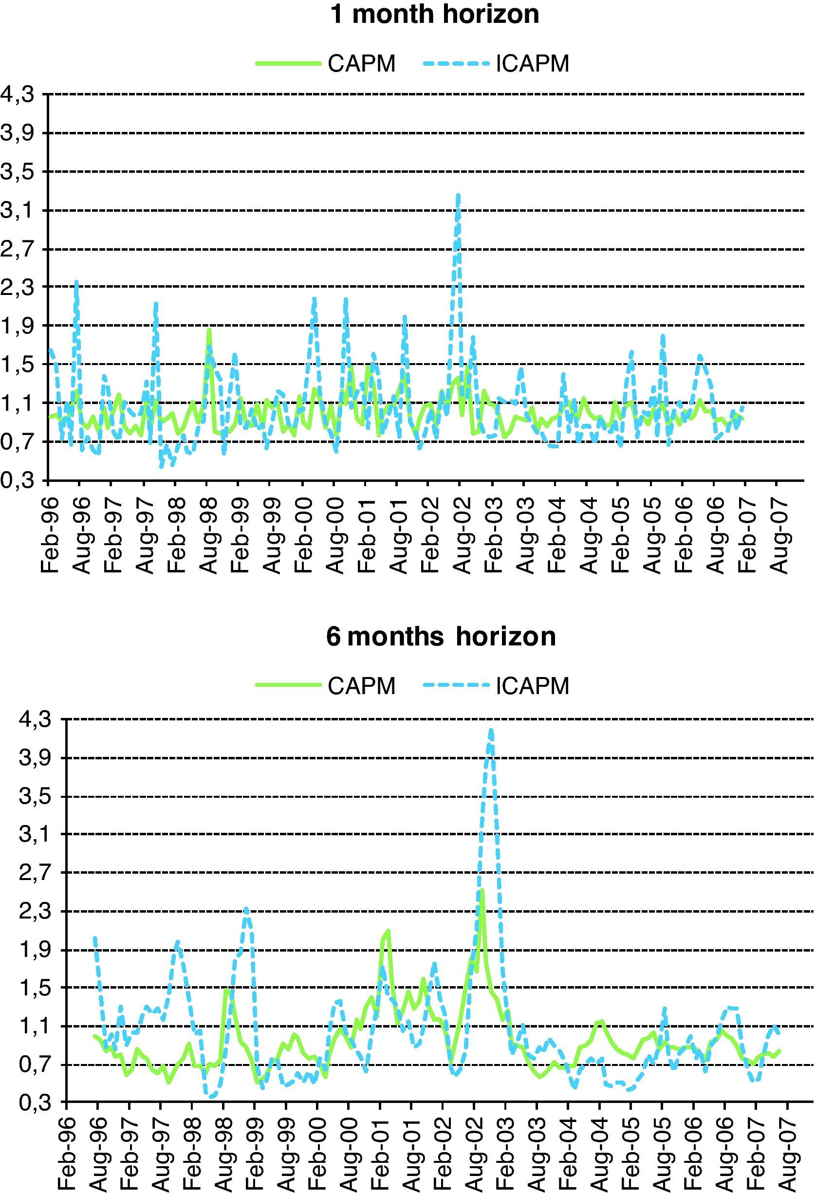
As an alternative way to compare the two model specifications, we now compute the time series for the SDFs obtained with the parameters estimated with an identity weighting matrix. To capture the strong cross-sectional and time-series variation of expected returns, we need a SDF with enough volatility. Moreover, its volatility should be high at the beginning of recessions and low when expansion periods begin. Fig. 2 shows the time-series of estimated SDFs for the two asset pricing models, for the one- and six-month horizons. At the shortest maturity, the SDF for the one-factor model becomes more volatile and with higher peaks in declining stock market periods once we add the variance risk premium as the second factor. This contribution of the variance risk premium is consistent with the relatively best results provided by the variance risk premium-based ICAPM relative to the one factor model in Table 2. At the six-month horizon, adding the variance risk premium again increases the volatility of the estimated SDF, relative to the one-factor model. This extensive representation of the SDF over the whole sample seems quite revealing of the difference between the two specifications. Furthermore, the reduction in MAPE indicates that the increased volatility in SDF actually helps pricing the portfolios in our sample.

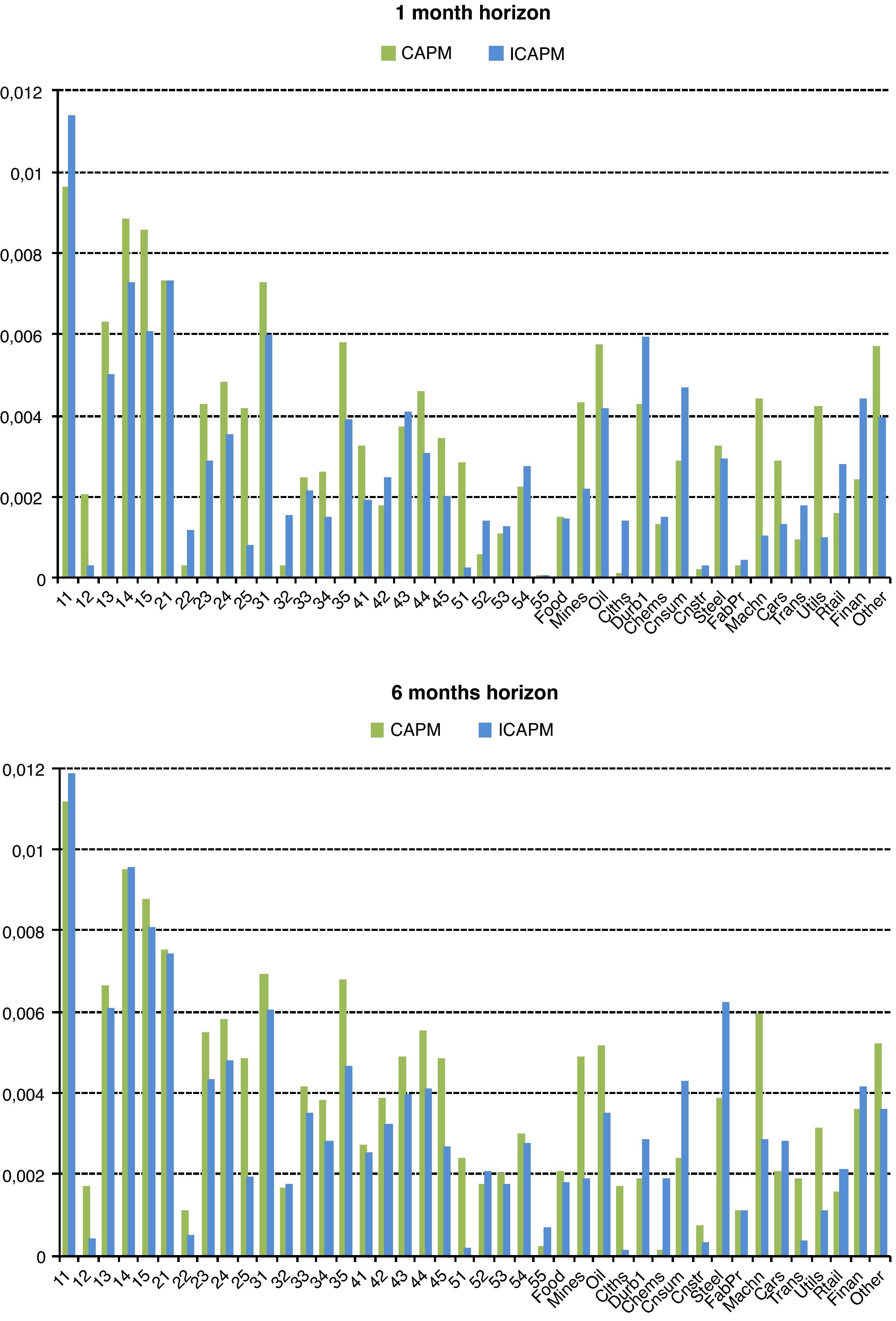
Independently of the non-concluding global evaluation of the model through the J-test, it is worthwhile to examine the model ability to explain portfolio prices in detail. We now describe which specific portfolios the model is more able to price correctly. Fig. 3 shows the average over time of the absolute pricing errors (APE) for each of the 42 original portfolios at the one- and six-month horizons, under the CAPM as well as under the ICAPM specification that incorporates the variance risk premium. When we add the variance risk premium to the one-factor model, the APE is reduced for most of the 42 portfolios considered. More specifically, the two-factor model reduces the APE for three out of the five extreme growth portfolios, FF31, FF41, and FF51 at both horizons. Interestingly, this is not the case for FF11, the portfolio of growth and small assets, whose performance shows a higher APE, or for the FF21 portfolio, whose pricing errors are essentially equal under the two specifications. It is also important to point out that the variance risk premium consistently helps pricing the extreme value Fama–French portfolios (FF15, FF25, FF35, and FF45).12 Finally, at the one-month horizon, the ICAPM achieves a better fit for portfolios FF12 throughout F15 (smallest assets) than the one-factor model. This evidence therefore suggests that the VRP factor contributes to an improvement in pricing extreme value, extreme growth and small-firm portfolios. Regarding industry portfolios, it turns out that adding the variance risk premium leads to a smaller APE for Mines, Oil, Machinery and Utilities at both horizons. Uncovering the characteristics of these sectors that provide a better fit in prices remains an interesting issue for further research.
5.2The linear version of the two-factor ICAPM
Estimating a tight theoretical model with a relatively short time series data can easily lead to a significant loss of efficiency in estimation that may condition the results of the tests for model adequacy. Despite the fact that the VRP seems to contain significant incremental information when pricing the cross-section of our test portfolios, especially at the shortest horizon, it should be recognized that the estimated coefficient of the VRP at this horizon is obtained with a large standard error. This consideration moves us to analyze in this section the pricing results obtained for the 25 Fama–French and the 17 industry portfolios under the linear beta representation of Eq. (7) for the one-month horizon. We therefore perform the well known Fama and MacBeth (1973) two-pass cross sectional analysis in which the monthly cross-sectional regressions are given by:

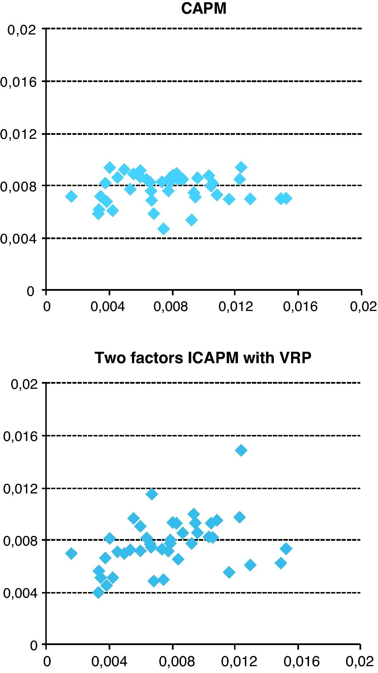
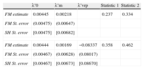
The results are presented in Table 3. Columns 1–3 report the risk premia estimates, together with the Fama–MacBeth and Shanken's (1992) standard errors. Columns 4 and 5 provide two pseudo-R2 statistics based on the residual sum of squares of the cross-sectional regressions. The coefficient associated with the variance risk premium beta turns out not to be statistically different from zero.13 But as in the non-linear model, it looks as if this could be more a consequence of estimating the risk premium for the variance swap payoff with low precision, since the incorporation of the variance risk premium as hedging factor leads to an increase in the cross-sectional overall goodness of fit from 0.237 to 0.358, or from 0.334 to 0.462, depending upon the statistical measure we may employ. The better fit of the linear model after incorporating the variance risk premium can be clearly appreciated in the two graphs of Fig. 4, that contain fitted expected returns versus average realized returns for the 42 portfolios for the CAPM and the ICAPM. The largest revisions occur for the FF25 portfolio, and for the Steel and Mine industry portfolios. The variance risk premium also improves average pricing for the small-value Fama–French portfolios, FF14 and FF15, which is consistent with the evidence reported on the GMM estimates.
Estimates and standard errors of intercepts and risk premia for the traditional Fama–MacBeth two-pass cross-sectional regressions, monthly data, January 1996 to January 2007.
| λˆ0 | λˆm | λˆvrp | Statistic 1 | Statistic 2 | |
| FM estimate | 0.00445 | 0.00218 | 0.237 | 0.334 | |
| FM St. error | (0.00475) | (0.00647) | |||
| SH St. error | [0.00475] | [0.00682] | |||
| FM estimate | 0.00444 | 0.00169 | −0.08337 | 0.358 | 0.462 |
| FM St. error | (0.00467) | (0.00628) | (0.08017) | ||
| SH St. error | [0.00467] | [0.00673] | [0.08670] | ||
This table presents the Fama–MacBeth two-step cross-sectional estimation results for the one-factor (CAPM) and two-factor (ICAPM) capital asset pricing models using the variance risk premium as the hedging factor:
Rjte=λ0+λmβjmt+λvrpβjvrpt+ujt.
The test assets are the returns on the 25 FF portfolios plus 17 industry portfolios in excess of the T-bill rate. We report risk premium parameter estimates (λˆ), standard errors under the Fama–MacBeth (FM) methodology in parenthesis, and the Shanken (SH) errors-in-variable-robust standard errors in brackets. The overall goodness of model fit is measured by the two following statistics:
Statistic 1:∑t=1T(TSSt−RSSt)∑t=1TTSSt;Statistic 2:1T∑t=1T1−RSStTSSt.
TSS and RSS denote the Total Sum of Squares and the Residual Sum of Squares, respectively.

Fitted expected returns vs. average realized returns. January 1996 to January 2007. This figure shows realized returns on the horizontal axis and fitted expected returns on the vertical axis for 25 size and book-to-market sorted portfolios and 17 industry portfolios. For each portfolio, the realized average return is the time-series average of the portfolio return, while the fitted expected return is the fitted value for the expected return from the corresponding model.
As suggested by our proposed SDF, stock returns should react very differently to the variance risk premium depending upon the state of the economy. In fact, as we already pointed out, the variance risk premium has very distinct compensation behavior for negative tail events. The previous non-significant cross-sectional results ignore the possibility of different conditional sensitivities of stock returns to the variance swap payoffs on “bad” versus “good” scenarios. We now want to analyze whether the actual information content of the variance risk premium occurs mainly during recessions.
In order to investigate this issue, we allow for market and variance risk premium betas to change over time as a function of the market state. We define factor regression regimes as a function of a given level of market returns, and estimate such threshold simultaneously with the betas for the market and the variance risk premium in each regime. In each regime we use the pooled data for the 42 portfolios for the corresponding periods. This is a Threshold Regression Model, which we estimate under the assumption of a Normal error term. The maximum likelihood estimate is the threshold level for which the least squares estimates of the regressions for the good and bad regimes lead to the lowest aggregate residual sum of squares:
where u is the market return threshold, and βm1, βvrp1, and βm2, βvrp2 are the market and variance risk premium betas for the regimes above and below the threshold, respectively.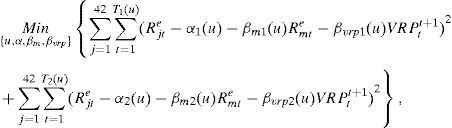
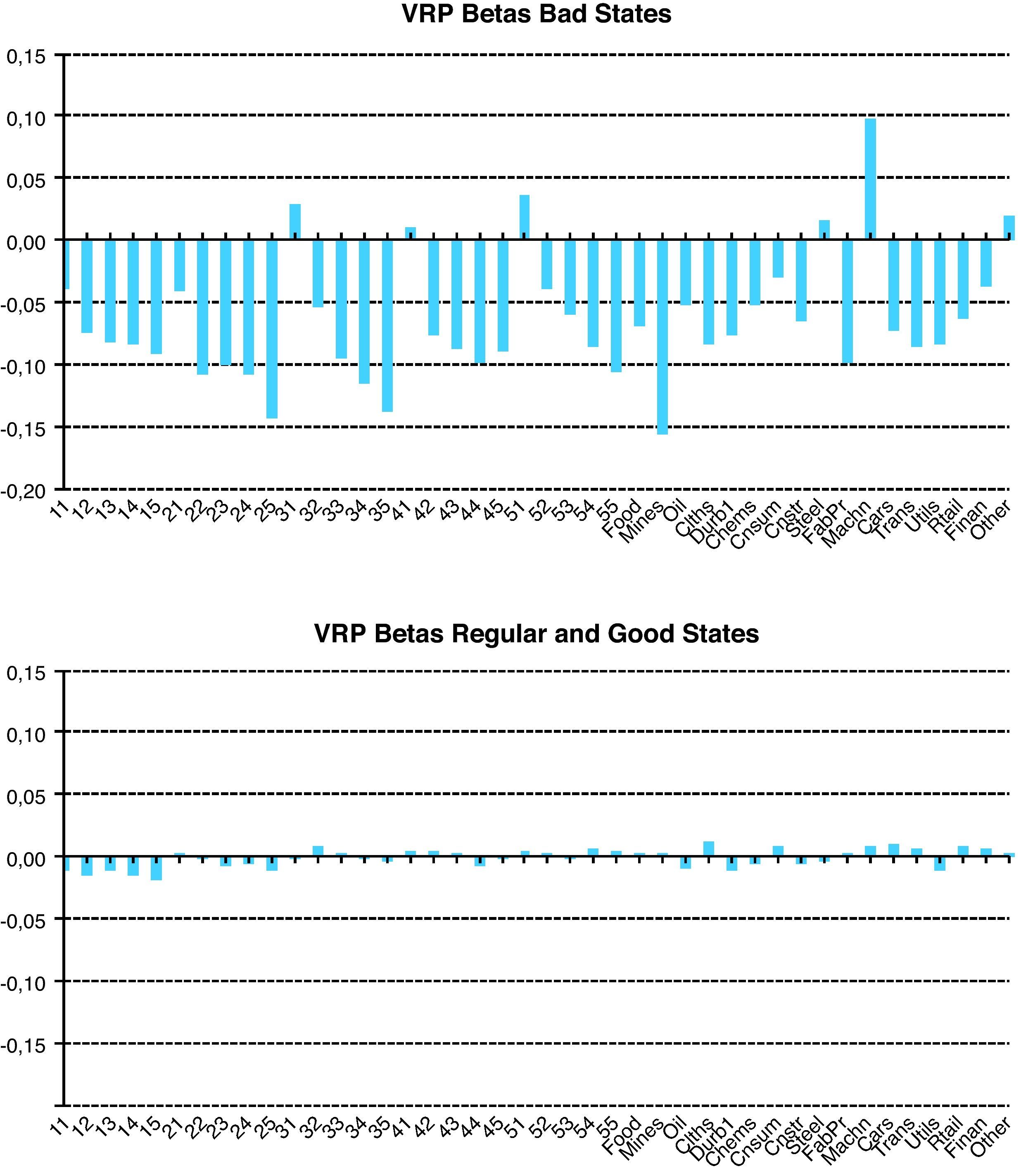
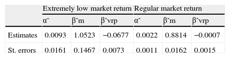
The maximum likelihood estimate of the market return threshold is −7.20%. This is an extreme return that splits the sample into “good/regular” regime for the 95% of the sample, and a “very low/very bad” regime that includes 5% of the sample. Given this partition, the results for the two-regime betas are reported in Table 4. The difference on the overall variance risk premium betas between both regimes are striking. The variance risk premium beta is highly significant and equal to −0.067. Since the variance risk premium is negative for most periods, long positions on variance swaps have positive payoffs only in those states in which the realized volatility is high enough to compensate the fears embedded in the risk neutral expectation of volatility. Moreover, it is also well known that volatility increases in periods of extremely low returns. This explains the large negative and highly significant variance risk premium beta in bad states. On the other hand, the variance risk premium beta for periods with positive or relatively small negative returns becomes practically zero. Even more illustrative is the evidence contained in Fig. 5 in which we present the variance risk premium betas for both regimes for each portfolio separately. For most portfolios, the variance risk premium betas become negative and large in bad states. However, they are practically zero in good and regular states. Interestingly, the extreme small-growth portfolios and construction have positive variance risk premium betas in bad states. This implies that the variance swap does not play its hedging role relative to these portfolios. It should be recalled that our sample period coincides with the boom in the real estate industry.
Estimates and standard errors of alphas and betas from a pooled OLS regression with two regimes based on a market return threshold, January 1996 to January 2007.
| Extremely low market return | Regular market return | |||||
| αˆ | βˆm | βˆvrp | αˆ | βˆm | βˆvrp | |
| Estimates | 0.0093 | 1.0523 | −0.0677 | 0.0022 | 0.8814 | −0.0007 |
| St. errors | 0.0161 | 0.1467 | 0.0073 | 0.0011 | 0.0162 | 0.0015 |
This table reports the overall market beta and the variance risk premium beta from a pooled OLS time-series regression under a two-regime specification defined by a given market return. The market return threshold is simultaneously estimated with the two regressions. The test assets are the 25 FF portfolios and 17 industry portfolios, with the returns in excess of the T-bill rate. The maximum likelihood estimate is the threshold level for which the least square estimates of the regressions for the good and bad regimes lead to the lowest aggregate residual sum of squares:
Min{u,α,βm,βvrp}∑j=142∑t=1T1(u)(Rjte−α1(u)−βm1(u)Rmte−βvrp1(u)VRPtt+1)2+∑j=142∑t=1T2(u)(Rjte−α2(u)−βm2(u)Rmte−βvrp2(u)VRPtt+1)2
where u is the market return threshold, and βm1, βvrp1, and βm2, βvrp2 are the market and the variance risk premium betas for the regime with the market return above and below the threshold, respectively.

Given this evidence, we now run the Fama–MacBeth two-pass cross sectional regressions using for the market return and the variance risk premium the appropriate betas for the market state in each period:
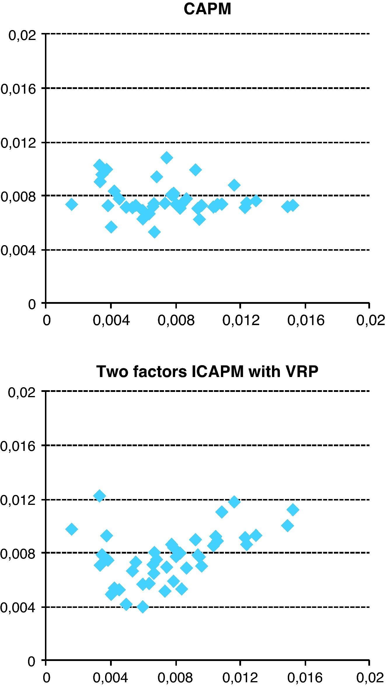
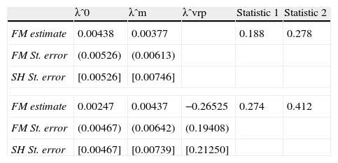
where βjmt+/− and βjvrpt+/− denote the betas in the appropriate “good” or “bad” states. As before, Fig. 6 shows a clear improvement in fit when we include the two-regime variance risk premium betas relative to the CAPM. More precisely, Table 5 reports the risk premia coefficients from the cross-sectional regression of expression (10). The compensation for the variance risk premium beta becomes much more negative than in Table 3 moving from −0.083 to −0.265 with a clear increase in precision. Moreover, the two measures of goodness of fit employed in the paper increase from 0.188 to 0.274 and from 0.278 to 0.412 when we add to the cross-sectional regression the variance risk premium betas conditional on the market threshold.

Fitted expected returns vs. average realized returns from cross-sectional regressions under two-regime betas based on a market return threshold. January 1996 to January 2007. This figure shows realized returns on the horizontal axis and fitted expected returns on the vertical axis for 25 size and book-to-market sorted portfolios and 17 industry portfolios. For each portfolio, the realized average return is the time-series average of the portfolio return, while the fitted expected return is the fitted value for the expected return from the corresponding model.
Estimates and standard errors of intercepts and risk premia for the market threshold two-regimes Fama–MacBeth two-pass cross-sectional regressions, January 1996 to January 2007.
| λˆ0 | λˆm | λˆvrp | Statistic 1 | Statistic 2 | |
| FM estimate | 0.00438 | 0.00377 | 0.188 | 0.278 | |
| FM St. error | (0.00526) | (0.00613) | |||
| SH St. error | [0.00526] | [0.00746] | |||
| FM estimate | 0.00247 | 0.00437 | −0.26525 | 0.274 | 0.412 |
| FM St. error | (0.00467) | (0.00642) | (0.19408) | ||
| SH St. error | [0.00467] | [0.00739] | [0.21250] | ||
This table presents the Fama–MacBeth two-step cross-sectional estimation results for the one-factor (CAPM) and two-factor (ICAPM) capital asset pricing models using the variance risk premium as the hedging factor:
Rjte=λ0+λmβjmt+/−+λvrpβjvrpt+/−+ujt,
where βjmt+/− and βjvrpt+/− denote the betas in the corresponding states.
The test assets are the 25 FF portfolios and 17 industry portfolios, with returns in excess of the T-bill rate. We report risk premia parameter estimates (λˆ), standard errors under the Fama–MacBeth (FM) methodology in parenthesis, and the Shanken (SH) errors-in-variable-robust standard errors in brackets. The overall goodness of model fit is measured by two statistics:
Statistic 1:∑t=1T(TSSt−RSSt)∑t=1TTSSt;Statistic 2:1T∑t=1T1−RSStTSSt.
TSS and RSS denote the Total Sum of Squares and the Residual Sum of Squares, respectively.
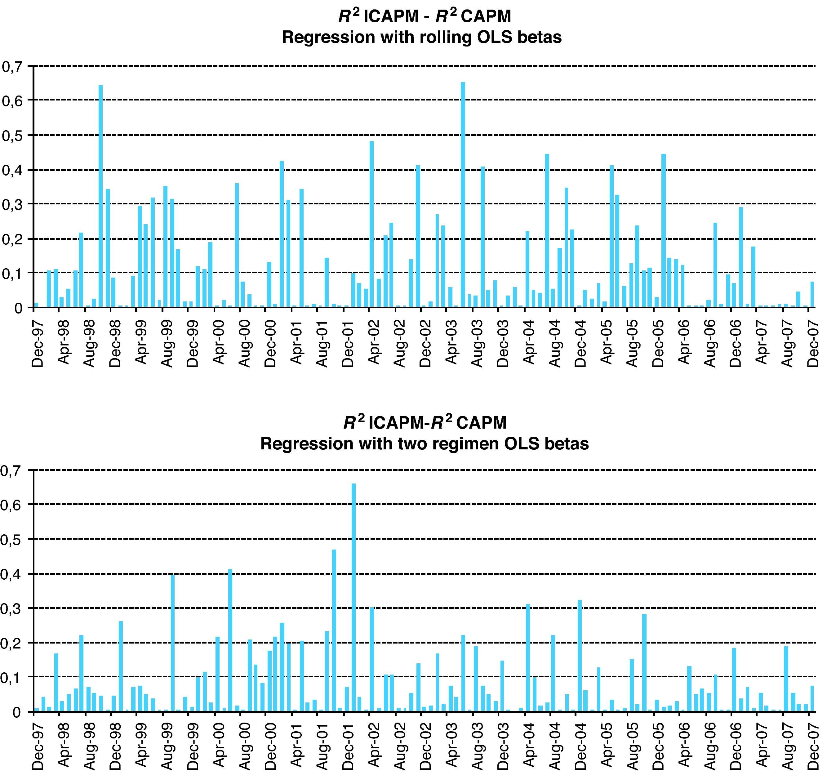
To summarize our findings, Fig. 7 contains the monthly differences between the adjusted R2 statistic from each Fama–MacBeth cross-sectional regressions with and without the variance risk beta as an explanatory variable. Independently of using a market threshold in the estimation of betas, we find an increase in the explanatory power of the two-factor ICAPM relative to the one-factor CAPM model in all months of our sample. We may therefore conclude that the variance risk premium contains incremental information for asset pricing over and above the market portfolio.
6Conclusions
Recent available evidence show that the excess return on the variance swap contract hedges equity market risks, interest rate and business cycle risks. This evidence motivates the consideration of a two-factor ICAPM with the variance risk premium playing the role of a hedging portfolio. The question is whether the variance risk premium acts as a sufficient statistic summarizing the information contained in a variety of risk indicators that might be potentially relevant for asset valuation.
Specification tests based on GMM estimates using the identity matrix as metric do not reject the model at one- and two-month horizons at conventional significance level, although the opposite is obtained at the remaining horizons. The time-varying behavior of the estimated SDF under the two-factor model presents a relatively more volatile behavior than the simple one-factor model, and pricing errors on individual portfolios are generally lower when the variance risk premium is incorporated into the model. More specifically, and relative to the one-factor model, the variance risk premium seems to explain small and value stocks, as well as Mines, Steel, Oil, Machinery, and Utilities. This is reflected in a reduction in global measures of fit between 16 and 18% for 1-, 6- and 12-month horizons, even though the reduced size of pricing errors does not seem to be small enough to not reject the model at these longer horizons according to the standard test for over-identification constraints. The linearized version of the model supports these results by providing a clearly improved fit to observed returns for the 25 Fama–French portfolios and the 17 industry portfolios, always at the one-month horizon.
Although it is standard practice, considering time-invariant parameter values for the full sample period might be too strong an assumption to make the model compatible with the data. When we include a recession threshold in the estimation of the variance risk premium betas in the linearized version of the model, we obtain that the compensation to the variance risk premium beta in asset pricing is limited to recession periods. Hence, the role of the variance risk premium as a pricing factor seems to concentrate on periods of significant market downturns. The cross-sectional overall measures of fit for the two-factor ICAPM relative to the one-factor CAPM specification increase independently of using conditional bad state betas or constant betas. The increase in monthly adjusted R2 in the cross sectional regression from adding the variance risk premium beta is often sizeable. Overall, our results suggest that the premium in variance swaps contains relevant information for asset pricing, possibly because summarizes information contained in a variety of macroeconomic and financial risk indicators. Analyzing the distinct gains in fitting prices of the different portfolios remains as an interesting issue for further research.
The authors acknowledge financial support from Ministerio de Ciencia e Innovación through grants ECO2008-02599/ECON (Belén Nieto), ECO2008-03058/ECON (Gonzalo Rubio), and SEJ2006-14354 (Alfonso Novales). Alfonso Novales and Gonzalo Rubio also acknowledge financial support from Generalitat Valenciana grant PROMETEO/2008/106 and from Programa Copernicus CEU-UCH/Banco de Santander. The authors thank seminar participants at the 33rd Meeting of the European Accounting Association, the 8th INFINITI Conference on International Finance, and XVII Foro de Finanzas, IESE, and especially Enrique Sentana, for constructive comments.
Let Rte be the N×1 vector of excess return of the N assets at time t and mt(θ) be one out of the two specifications of the SDFs described in Section 4, where θ is the vector of the preference parameters for each particular specification. We define an N×1 vector of moment conditions containing the pricing errors generated by the model at time t,
and the corresponding sample averages,
Then GMM estimator minimizes the following quadratic form
where WT is a weighting N×N matrix.
For estimation, we could use the optimal weighting matrix in Hansen (1982), ST−1, where
Instead of that, we employ a pre-specified weighting matrix which is either the identity matrix (for the results of Panel A of Table 2) or the matrix of the second moments of excess returns (for the results of Panel B of Table 2).
The asymptotic variance–covariance matrix of the GMM estimates is given by
where DT is a matrix of partial derivatives defined by
Then, the standard errors of the estimated coefficients θˆ are computed from the estimated variance:
where DˆT and SˆT are obtained replacing θ by θˆ in DT and ST, respectively.
The evaluation of the model performance is carried out by testing the null hypothesis:
with Dist=g(θ)′Wg(θ) where, as mentioned above, the weighting matrix, W, is either the identity matrix or the second moment matrix of excess returns.
If the weighting matrix is optimal, T[Dist(θˆ)]2 is asymptotically distributed as a Chi-square with N−P−1 degrees of freedom, where P is the number of parameters. However, for any other weighting matrix (including the identity matrix), the distribution of the test statistic is unknown. Jagannathan and Wang (1996) show that, in this case, T[Dist(θˆ)]2 is asymptotically distributed as a weighted sum of N−P−1 independent Chi-square random variables with one degree of freedom. That is
where λi, for i=1, 2,…,N−P−1, are the positive eigenvalues of the following matrix:in which X1/2 means the upper-triangular matrix from the Choleski decomposition of X, and IN is a N-dimensional identity matrix.
Therefore, in order to test the different models we estimate, we proceed in the following way. First, we estimate the matrix A by
and compute its nonzero N−P−1 eigenvalues. Second, we generate {vhi}, h=1, 2,…,100, i=1, 2,…,N+1−P, independent random draws from a χ2(1) distribution. For each h, uh=∑i=1N−P−1λivhi is computed. Then we compute the number of cases for which uh>T[Dist(θˆ)]2. Let p denote the percentage of this number. We repeat this procedure 1000 times. Finally, the p-value for the specification test of the model is the average of the p values for the 1000 replications.

