


The New Capital Accord (Basel II) proposes a minimum threshold of 10,000 Euros for operational losses when estimating regulatory capital for financial institutions. But since this recommendation is not compulsory for the bank industry, banks are allowed to apply internal thresholds discretionally. In this sense, we analyze the potential impact that the selection of a specific threshold could have on the final estimation of the capital charge for covering operational risk, adopting a critical perspective. For this purpose, by using the Internal Operational Losses Database (IOLD) provided by a Spanish Saving Bank, we apply the Loss Distribution Approach (LDA) for different modelling thresholds. The results confirm the opportunity cost in which banks can incur depending on the internal threshold selected. In addition, we consider that the regulatory threshold, established by the Committee, could result inadequate for some financial institutions due to the relative short length of the current IOLDs.
Among other methodologies proposed by the Basel Committee (2006) to estimate the operational risk regulatory capital, the Advanced Measurement Approach (AMA) is the strategic goal to which banks should evolve in order to reach a more efficient capital allocation. Within the AMA, the model with greater acceptance is the Loss Distribution Approach (LDA) which is theoretically described by Frachot et al. (2004a). Empirically this approach is applied by Moscadelli (2005) and Dutta and Perry (2006) to a European and American Banks sample, respectively. Inherited from actuarial sciences, the LDA generates a distribution of operational losses, from which to infer directly the Capital at Risk (CaR) as its 99.9 percentile. In this regard, to ensure a proper implementation and validation of the LDA, the Basel Committee (2006: 150) suggests the combined use of both internal and relevant external loss data, scenario analysis and bank-specific business environment and internal control factors. Similarly, the Committee (2006: 153) suggests a minimum threshold of 10,000 Euros for the collection. However, due to the current scarcity of the internal operational loss data recorded by banks, Basel II offers the possibility that the financial institution could define that cut-off level. The main aim of data left-truncating is not only to avoid difficulties with collection of insignificant losses, but also to focusing on those events located at the tail of the distribution. The impact of establishing cut-off levels in operational risk has been addressed by Baud et al. (2002), Chernobai et al. (2006), Mignola and Ugoccioni (2006), Luo et al. (2007) and Shevchenko and Temnov (2009). In particular, Chernobai et al. (2006), analyze the treatment of incomplete data when applying threshold levels. They prevent us to incur in unwanted biases by highlighting the serious implications on the operational capital charge relevant figures, if not duly addressed. Furthermore, these authors propose to reconstruct the shape of the lower part of the distribution by fitting the collected data and extrapolating down to zero. By doing so, in addition to avoiding the information loss carried by the missing data, one would be able to produce accurate estimates of the operational capital charge.
In the opposite, Mignola and Ugoccioni (2006) state, by conducting a laboratory set-up, that operational risk measures are insensitive to the presence of a collection threshold up to fairly high thresholds. Moreover, the reconstruction of the severity and frequency distributions below threshold introduces the assumption that the same dynamics drives both small and intermediate losses. The study conducted by Mignola and Ugoccioni (2006) concludes that such reconstruction is an unnecessary and unjustified burden. A simpler approach consisting in describing correctly only the data above threshold can be safely adopted.
On this basis, we carry out an empirical analysis with the objective to test the effect of different cut-off levels on statistical moments of the loss distribution and analyzing its potential impact on Capital at Risk (CaR), discriminating between lower and upper thresholds. For this purpose, we start doing an Exploratory Data Analysis (EDA) on the Internal Operational Loss Database (IOLD), provided by a saving bank. Secondly, the methodological approach (LDA) is described step by step. Finally, the results are presented by emphasizing the importance of the threshold selection in the final determination of capital charge for upper cut-off levels.
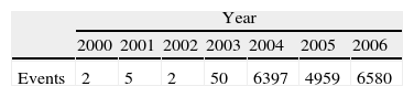
2Data and methodology2.1The dataIn order to conduct our analysis we have used, as said before, the Internal Operational Loss Database (IOLD) provided by a medium-sized Spanish Saving Bank that operates within the retail banking sector. The sample comprises 7 years of historical operational losses. In Table 1, the number of events recorded per year is given.
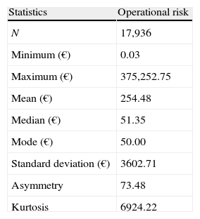
As illustrated in Table 1, the frequency of events from 2000 to 2003 is not significant. Consequently, for avoiding the distortion of the frequency distribution, we shall consider only the representative years 2004, 2005 and 2006. It should also be noted that inflation, affecting the data for the years over which they are compiled, can distort the results of the research. To take this effect into account, we have used the CPI (Consumer Prices Index) to adjust the amount of the losses, taking the year 2006 as the base. Thus we have converted the nominal losses into equivalent monetary units. As Tukey (1977) suggests, before implementing any statistical approach, it is essential to perform an Exploratory Data Analysis (EDA) of the data set by analyzing the nature of the sample used, as presented in Table 2.
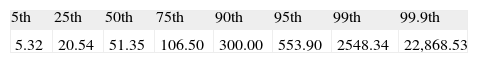
From Table 2, the observed values for the shape parameter indicate a positive asymmetry and leptokurtosis. At the same time, it should be noted that the mean is much higher than the median, pointing out the positive asymmetry of the loss distribution. In a broad sense, the operational losses are characterized by a grouping, in the central body, of low severity values, and a wide tail marked by the occurrence of infrequent but extremely onerous losses. This characteristic can be observed very clearly by considering the percentiles of the operational risk distribution (see Table 3).
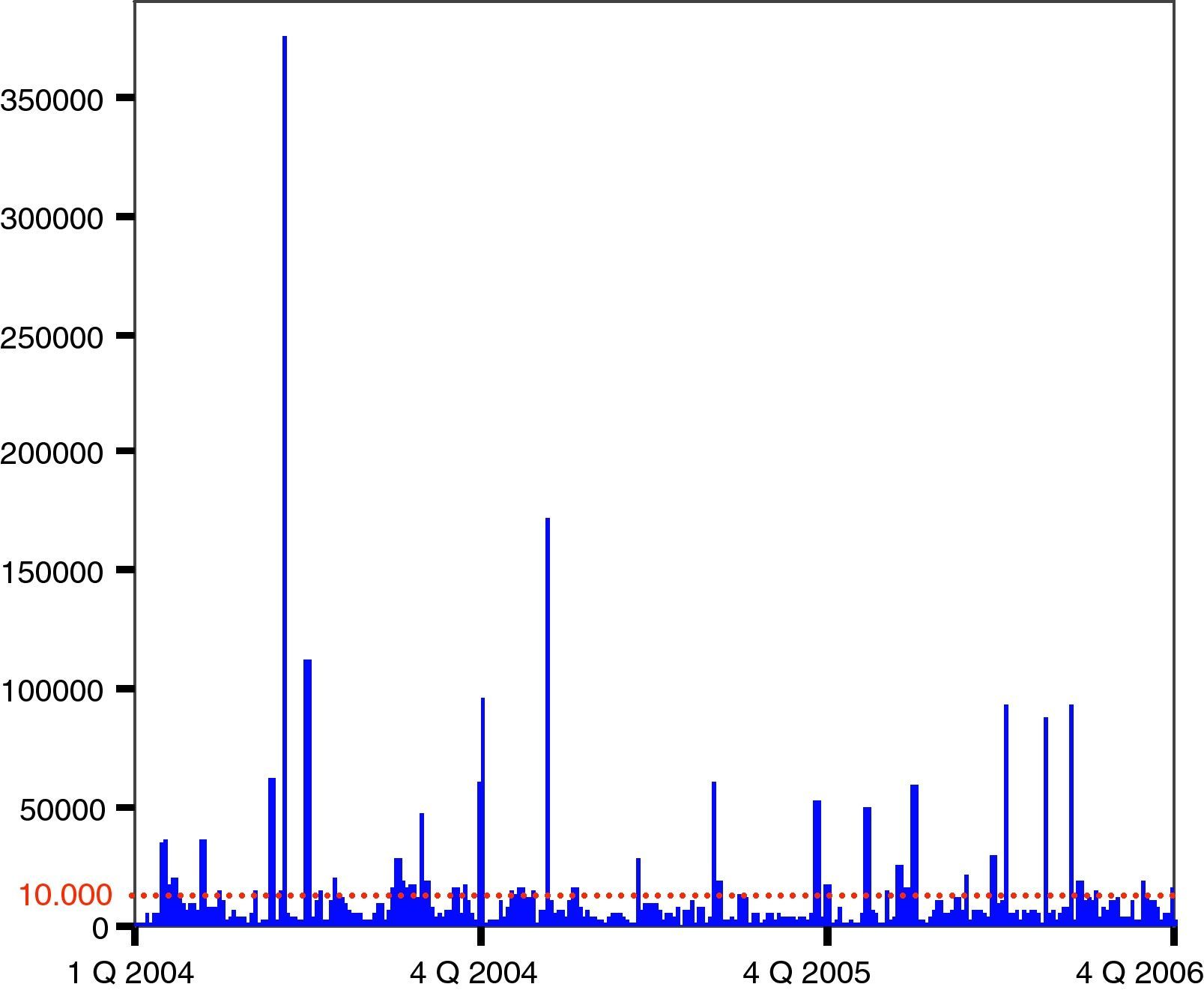
It is remarkable, from Table 3 that 99% of the losses recorded in the IOLD are below 2548.34 Euros, so if we were to apply the regulatory threshold of 10,000 Euros, we would reject most of the data available (see Fig. 1).

Having truncated the sample at the regulatory level, we finally count for 43 exceedances. In this sense, according to McNeil and Saladin (1997), we should ensure at least 25 peaks over the threshold to gain statistical robustness; anything below such a number the results would not be reliable. Although 200 excesses would be ideal, from 50 to 100 we can reach to realistic situations.
2.2The methodologyFollowing the Committee recommendations, we have chosen the LDA when estimating the capital charge for operational risk. This advanced approach is a statistical technique based on the information of historical losses, from which to obtain the distribution of aggregate losses. For the calculation of the regulatory capital the concept of Operational Value at Risk (OpVaR) is applied. In short, we can interpret the OpVaR as a figure, expressed in terms of monetary units that informs us about the maximum potential loss that an entity could incur due to operational risk during one year, and with a level of statistical confidence of 99.9% (Basel, 2006). When addressing operational losses is essential to define two parameters: frequency and severity.
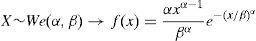
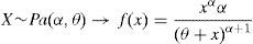
2.2.1Severity distributionThe severity (X) is defined from a statistical point of view as a random continuous variable that represents the amount of loss (see Böcker and Klüppelberg, 2005). Although the normal hypothesis is commonly considered for market risk modelling, the shape variable (see Table 2) shows an empirical operational risk distribution very far from the expected Gaussian distribution. Assuming the absence of normality, and following Moscadelli (2005), we have tested three probabilistic functions: Lognormal (LN), Weibull (We) and Pareto (Pa), in terms of its kurtosis. Ranked on this basis, the Weibull function is commonly used for distributions with smooth tail; the Lognormal is suitable for distributions with moderate or average tail; and, for those with heavy tail, the Pareto function is strongly recommended.
In order to calibrate the Goodness of Fit (GOF), we apply the Kolmogorov–Smirnov (K–S) test, which is appropriated for continuous variables. The specific values of the parameters for each distribution are estimated by Maximum Likelihood (ML). The probabilistic models are defined statistically as follows:
2.2.2Frequency distribution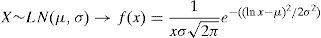
On the contrary, the frequency is a random discrete variable (N) that symbolizes the number of events occurring during a time horizon of one year. In other words, it represents the probability that the event may happen. The Poisson (Po) distribution – used successfully in actuarial techniques for insurance1 – is recommended for modelling such a variable due to its potential advantages (see Fontnouvelle et al., 2005). This function is characterized by one single parameter, lambda (λ), which represents, on average, the number of events occurring in one year, that is:
2.2.3Aggregate loss distribution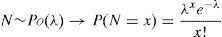
Once the distributions of severity and frequency have been characterized separately, the last step of the methodological procedure consists of obtaining a third distribution, that is, the aggregate loss distribution. Thus, the total loss associated (S) will be given by:

This amount is therefore of what is computed from a random number of loss events, with values that are also random, under the assumption that the severities are independent of each other and, at the same time, independent of the frequency (Frachot et al., 2004b). The aggregate loss function G(x), is obtained by convolution. This is a mathematical procedure that transforms the distributions of frequency and severity into a third one by the superposition of both distributions (Feller, 1971: 173). For this purpose we have conducted the Monte–Carlo Simulation (see Klugman et al., 2004: chap. 17). Once the aggregate distribution function has been determined, we are ready to calculate the Capital at Risk (CaR) for operational risk by applying the 99.9th percentile of such distribution, that is:

In a broad sense, according to the Committee (2006: 151), the regulatory capital (CaR) should cover both the expected (EL) and the unexpected loss (UL). In that case, the CaR and the OpVaR are identical2; see formula (6).
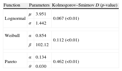
3Empirical results3.1Fitting the severity distributionIn general, we have to differentiate between capturing-threshold and modelling-threshold. To some extent, the second one is conditioned by the former. Since our database does not include any specific threshold, henceforth our benchmark will be defined by the 0 Euros level. In Table 4, the parameter estimates and the GOF are presented for each probabilistic model tested.
GOF for the benchmark threshold.
| Function | Parameters | Kolmogorov–Smirnov D (p-value) | |
| Lognormal | μ | 3.951 | 0.067 (<0.01) |
| σ | 1.442 | ||
| Weibull | α | 0.854 | 0.112 (<0.01) |
| β | 102.12 | ||
| Pareto | α | 0.134 | 0.462 (<0.01) |
| θ | 0.030 | ||
In this table the results of K–S test are reported for the different severity probabilistic models, assuming a 0 Euros cut-off level. As noticed, all of them present low statistical significance (below 1%). In particular, the Lognormal distribution provides the lower gap in the K–S statistic (D), followed by the Weibull and the Pareto functions, in this order. Since the statistic value represents, in absolute terms, the maximum distance between the observed distribution and the theoretical one, the lower value of D, the better fit. In consequence, the Lognormal appears to be the most suitable probabilistic function.
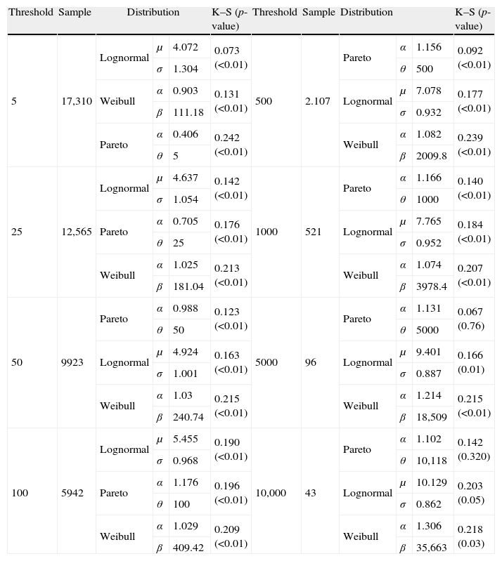
For calibrating the threshold effect when modelling operational losses, we have defined discretionally, eight different thresholds (5, 25, 50, 100, 500, 1000, 5000, and 10,000 Euros).
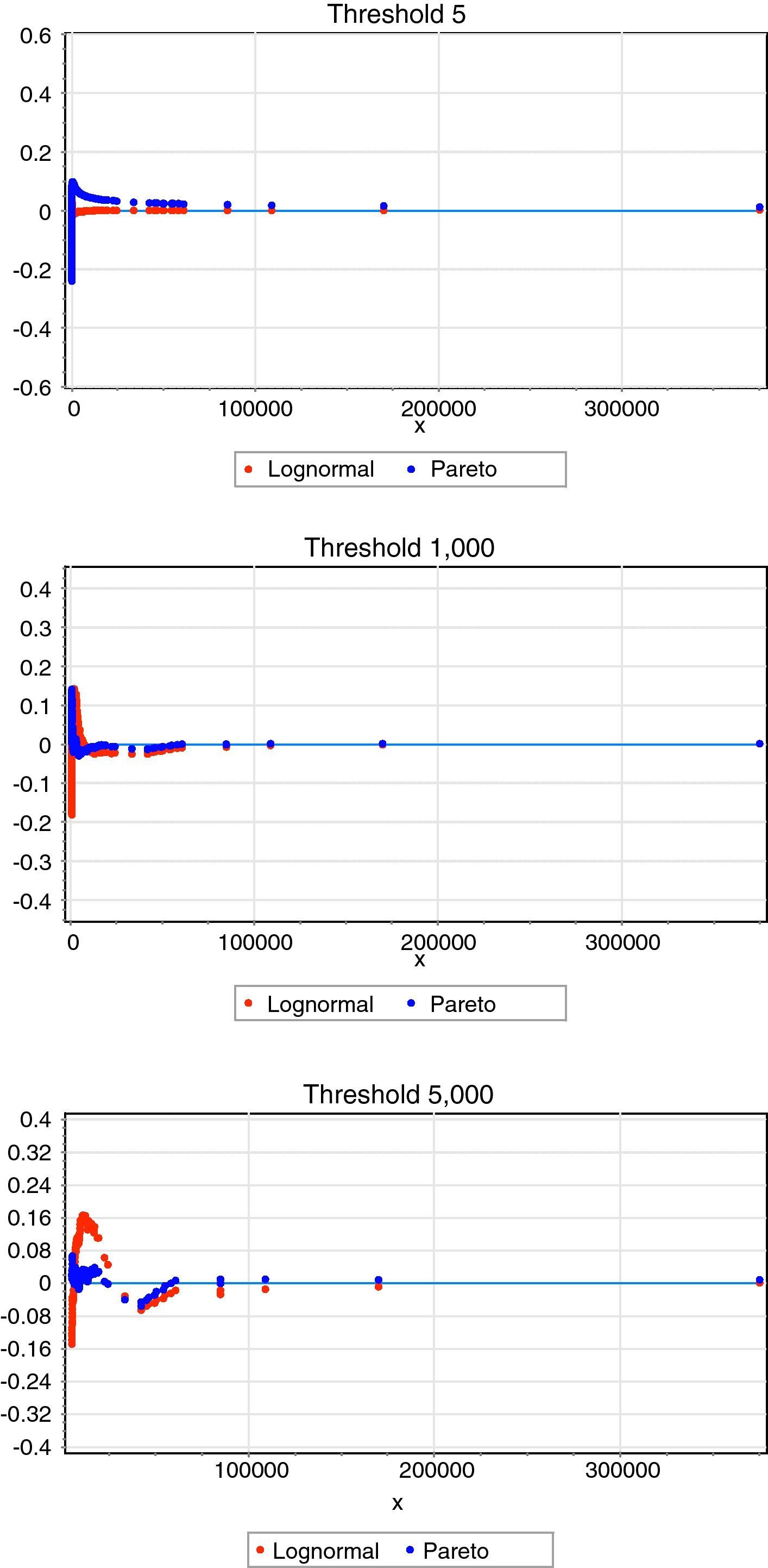
As Table 5 illustrates, in general, when using lower thresholds, the Lognormal distribution appears to be the most suitable distribution. On the contrary, for higher levels, in particular from the 100 Euros threshold onwards, the Pareto function provides a much better adjustment to the empirical data. To reinforce this conclusion we have drawn the same in Fig. 2.
GOF for different thresholds.
| Threshold | Sample | Distribution | K–S (p-value) | Threshold | Sample | Distribution | K–S (p-value) | ||||
| 5 | 17,310 | Lognormal | μ | 4.072 | 0.073 (<0.01) | 500 | 2.107 | Pareto | α | 1.156 | 0.092 (<0.01) |
| σ | 1.304 | θ | 500 | ||||||||
| Weibull | α | 0.903 | 0.131 (<0.01) | Lognormal | μ | 7.078 | 0.177 (<0.01) | ||||
| β | 111.18 | σ | 0.932 | ||||||||
| Pareto | α | 0.406 | 0.242 (<0.01) | Weibull | α | 1.082 | 0.239 (<0.01) | ||||
| θ | 5 | β | 2009.8 | ||||||||
| 25 | 12,565 | Lognormal | μ | 4.637 | 0.142 (<0.01) | 1000 | 521 | Pareto | α | 1.166 | 0.140 (<0.01) |
| σ | 1.054 | θ | 1000 | ||||||||
| Pareto | α | 0.705 | 0.176 (<0.01) | Lognormal | μ | 7.765 | 0.184 (<0.01) | ||||
| θ | 25 | σ | 0.952 | ||||||||
| Weibull | α | 1.025 | 0.213 (<0.01) | Weibull | α | 1.074 | 0.207 (<0.01) | ||||
| β | 181.04 | β | 3978.4 | ||||||||
| 50 | 9923 | Pareto | α | 0.988 | 0.123 (<0.01) | 5000 | 96 | Pareto | α | 1.131 | 0.067 (0.76) |
| θ | 50 | θ | 5000 | ||||||||
| Lognormal | μ | 4.924 | 0.163 (<0.01) | Lognormal | μ | 9.401 | 0.166 (0.01) | ||||
| σ | 1.001 | σ | 0.887 | ||||||||
| Weibull | α | 1.03 | 0.215 (<0.01) | Weibull | α | 1.214 | 0.215 (<0.01) | ||||
| β | 240.74 | β | 18,509 | ||||||||
| 100 | 5942 | Lognormal | μ | 5.455 | 0.190 (<0.01) | 10,000 | 43 | Pareto | α | 1.102 | 0.142 (0.320) |
| σ | 0.968 | θ | 10,118 | ||||||||
| Pareto | α | 1.176 | 0.196 (<0.01) | Lognormal | μ | 10.129 | 0.203 (0.05) | ||||
| θ | 100 | σ | 0.862 | ||||||||
| Weibull | α | 1.029 | 0.209 (<0.01) | Weibull | α | 1.306 | 0.218 (0.03) | ||||
| β | 409.42 | β | 35,663 | ||||||||
In this table we fit the truncated severity distributions after applying different thresholds. The size of sample is also reported, decreasing till 43 observations for the regulatory cut-off level. For this particular case, we observed how the Pareto function gathers statistical robustness against the Lognormal.
 and the theoretical one, by considering three different thresholds (5, 1000 and 5000 Euros, respectively). For the lower threshold (5 Euros) the Lognormal distribution is the best candidate for modelling operational losses, whereas as we increase the threshold level there is a clear trade off with the Pareto function.")
Probability difference graph. In this figure, we have plotted the probability difference graph to capture the difference between the empirical Cumulative Distribution Function (CDF) and the theoretical one, by considering three different thresholds (5, 1000 and 5000 Euros, respectively). For the lower threshold (5 Euros) the Lognormal distribution is the best candidate for modelling operational losses, whereas as we increase the threshold level there is a clear trade off with the Pareto function.
As our primary objective is to assess the cut-off level effect on CaR, we have finally decided to address it in isolation. For this purpose, following the Basel Committee (2001) suggestions, we have used the LDA-Standard as a benchmark, that is, Lognormal distribution for modelling the severity and the Poisson distribution for the frequency. Thus, for example, the Weibull Function, which presents a thinner tail, would give rise to a lower capital charge; whereas the Pareto function, more sensitive to leptokurtosis, could increase the final CaR, beyond the threshold effect itself. Consequently, we are going to assume Lognormal function whatever the case is.
3.2Fitting the frequency distributionWhen a cut-off level is set, the average number of reported events is reduced. It doesn’t imply lower capital consumption necessarily, since the number of recorded events, on average, does not represent the real risk exposure. In other words, the observed data captures partially the risk exposure. Consequently, the real frequency is higher than the observed one, since the latter is related to those losses beyond the minimum. Consequently, as Frachot et al. (2004a) state, the average number of events must be corrected for avoiding bias, see formula (7).
where the “true” frequency, λ, is equal to the ratio between the observed frequency, λSample, and the probability of occurrence beyond the threshold, T. Thus, the calibration of the frequency distribution needs a previous estimation of the truncated severity distribution parameters.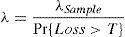
Assuming the LDA-Standard, if Lognormal distribution is proposed for severity we can rewrite the previous equation as follows:
where F(T; μ, σ) represents the Lognormal probability distribution function, F(x), μ is the scale parameter and σ the shape parameter, that is, P(X≤x).3.3Capital at Risk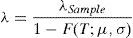
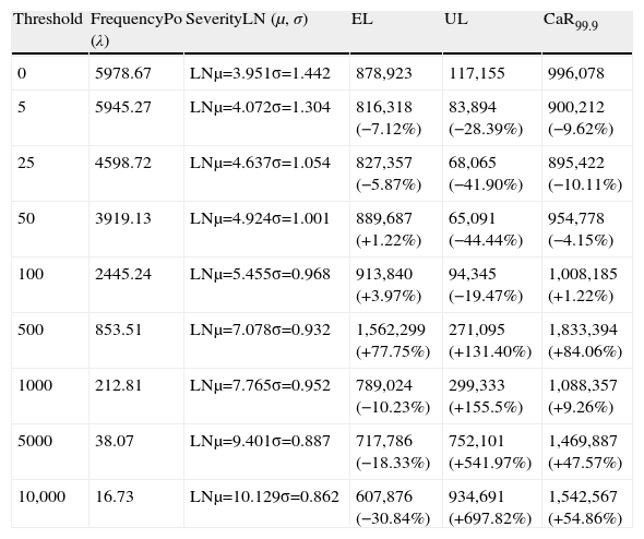
Assuming the LDA-Standard approach, the capital charge is finally obtained once we have modelled the frequency and the severity through the convolution process. Embrechts et al. (2003) endorse McNeil and Saladin's (1997) study, this time using lognormally distributed operational losses and reaching the same conclusions about the convenience of ensuring at least 25 exceedances beyond the threshold to obtain much more reliable statistical results. As Table 6 illustrates, we have estimated the Capital at Risk (CaR99.9) as well as the expected loss (EL) and the unexpected loss (UL) for the established thresholds.
Capital at Risk (CaR), expected loss (EL) and unexpected loss (UL).
| Threshold | FrequencyPo (λ) | SeverityLN (μ, σ) | EL | UL | CaR99.9 |
| 0 | 5978.67 | LNμ=3.951σ=1.442 | 878,923 | 117,155 | 996,078 |
| 5 | 5945.27 | LNμ=4.072σ=1.304 | 816,318 (−7.12%) | 83,894 (−28.39%) | 900,212 (−9.62%) |
| 25 | 4598.72 | LNμ=4.637σ=1.054 | 827,357 (−5.87%) | 68,065 (−41.90%) | 895,422 (−10.11%) |
| 50 | 3919.13 | LNμ=4.924σ=1.001 | 889,687 (+1.22%) | 65,091 (−44.44%) | 954,778 (−4.15%) |
| 100 | 2445.24 | LNμ=5.455σ=0.968 | 913,840 (+3.97%) | 94,345 (−19.47%) | 1,008,185 (+1.22%) |
| 500 | 853.51 | LNμ=7.078σ=0.932 | 1,562,299 (+77.75%) | 271,095 (+131.40%) | 1,833,394 (+84.06%) |
| 1000 | 212.81 | LNμ=7.765σ=0.952 | 789,024 (−10.23%) | 299,333 (+155.5%) | 1,088,357 (+9.26%) |
| 5000 | 38.07 | LNμ=9.401σ=0.887 | 717,786 (−18.33%) | 752,101 (+541.97%) | 1,469,887 (+47.57%) |
| 10,000 | 16.73 | LNμ=10.129σ=0.862 | 607,876 (−30.84%) | 934,691 (+697.82%) | 1,542,567 (+54.86%) |
Under the so-called LDA-Standard, we obtain different CaR figures depending on the threshold selected. Moreover, we have split up the final capital charge in terms of expected (EL) and unexpected loss (UL) in order to obtain further conclusions. The results for each cut-off level are compared to the benchmark threshold, which has been set at 0 Euros. The final impact on CaR, EL and UL is reported in relative terms.
For the threshold interval, between 5 and 50 Euros, we find a significant reduction in the resulting CaR. As long as the parametric characterization of the severity distribution is very similar to that estimated using a 0 Euros threshold, the frequency of events is reduced given rise to a lower capital charges than the benchmark. When 100 Euros cut-off level is set, the corresponding CaR is very close to the benchmark. Despite of decrease experienced by the frequency, in the convolution process, the increase in the scale of the severity provokes a compensation effect on the final CaR.
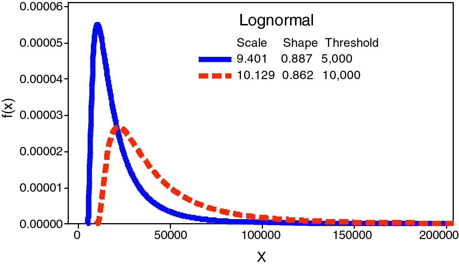
For upper thresholds, from 500 Euros onwards, we observe a huge increase of the UL in comparison to the benchmark. This is due to the stress on the scale parameter – the mean and the variance – of the severity distribution. In the case of the regulatory threshold, it is remarkable that the UL increases to 697.82% whereas the frequency has declined to 16.73, on annual average. This fact brings into light the higher weight of the severity against the frequency distribution in the LDA model and, in consequence, in the final capital charge. Fig. 3 illustrates such effect on the Lognormal distribution.
4Conclusions
In this paper, we have developed an empirical analysis, based on an IOLD, in order to test the CaR sensitiveness to different thresholds, including the regulatory cut-off level. From the modelling process, we find that the Lognormal function provides a better fit for lower cut-off levels. In contrast, for upper levels the lower density of the central body of the distribution makes the test for the adjustment more sensitive to the tails, to which the Pareto distribution seems to be more precise. In short, it is demonstrated that for higher thresholds this probabilistic model gains statistically significance. But we should warn that the Pareto shape parameter estimates in most of the cases provide with infinite statistical moments (2nd, 3rd, and 4th), that is, variance, asymmetry and kurtosis, what would lead us to unrealistic capital charges.
By applying the LDA-Standard (Poisson and Lognormal), we observe how different the response of the frequency and the severity distributions are as the threshold level raise. The increase in the threshold provokes a right handed shift of the distribution on the X-axis, and consequently increasing both operational losses distribution's position and dispersion measures. Furthermore, since the convolution process consists of mixing frequency and severity distributions up, the CaR experiences a spectacular growth when the cut-off level is stressed due to relative weight of the severity, against the frequency, within the LDA model. The results confirm the opportunity cost in which banks may incur depending on the internal threshold selected. Although, we consider that the regulatory threshold, 10,000 Euros, could be inadequate for some financial institutions or business lines, for which the internal data were not sufficient to obtain robust or, at least, realistic results. In consequence, we suggest that cut-off levels should vary somewhat among banks, and even within business lines or event types.
This study has been financed by the Consejería de Innovación, Ciencia y Empresa of the Junta de Andalucía (Regional Government of Spain), through the call for Projects of Excellence 2007. Reference PO6-SEJ01537. The authors acknowledge the helpful suggestions of Professor Aman Agarwal from Indian Institute of Finance, at the 9th International Scientific School MASR Saint Petersburg (Russia) and the comments received in both the 11th Spanish-Italian Congress of Financial and Actuarial Mathematics and the 17th Forum Finance.

