


This paper introduces a coincident indicator of systemic liquidity risk in the Italian financial markets. In order to take account of the systemic dimension of liquidity stress, standard portfolio theory is used. Three sub-indices, that reflect liquidity stress in specific market segments, are aggregated in the systemic liquidity risk indicator in the same way as individual risks are aggregated in order to quantify overall portfolio risk. The aggregation takes account of the time-varying cross-correlations between the sub-indices, using a multivariate GARCH approach. This is able to capture abrupt changes in the correlations. We evaluate the indicator on its ability to match the results of a survey conducted among financial market experts to determine the most liquidity stressful events for the Italian financial markets. The results show that the systemic liquidity risk indicator accurately identifies events characterized by high systemic risk.
The financial crisis has underscored the importance of timely and effective measures of systemic risk. Academics, central banks and international organizations are currently devoting much time and effort to developing tools and models which can be of help in monitoring, identifying and assessing potential threats to the stability of the financial system. This paper contributes to this strand of the literature by introducing an indicator of systemic liquidity risk in the Italian financial markets.1
In this regard the recent financial crisis has shown that market liquidity can suddenly deteriorate dramatically. Liquidity changes over time for individual securities and for the market overall. As pointed out by Amihud et al. (2013), liquidity varies for a number of reasons. First, it depends in part on the transparency of information about a security's value, which can change over time. Second, the number of liquidity providers and their access to capital is an important determinant of liquidity as argued by Brunnermeier and Pedersen (2009). When liquidity providers (such as banks, market makers, trading firms and hedge funds) lose capital and their access to securitized funding is constrained, as in 2008, they provide less liquidity as their risk aversion increases. Consequently, market liquidity drops simultaneously for most securities and market segments.
Liquidity can also suddenly dry up because of externalities. The willingness to trade by the sell-side facilitates trading for investors (the buy-side) and, consequently, potentially improves market liquidity. It stands to reason that a decreased willingness to trade reduces market liquidity and, if persistent, can exacerbate the liquidity shortfall in the market by triggering a downward spiral that will affect asset prices and thus increase risk aversion. In addition, increased uncertainty makes the provision of liquidity riskier and increases the reward that liquidity providers demand, that is, the cost of trading increases.
In order to address some of these issues, this paper introduces an indicator of liquidity stress using data on the Italian financial markets. The main aim of stress indices is to measure the current level of frictions and strains (or their absence) in the financial system and to summarize it in a single statistic. The proposed indicator is a coincident risk indicator which permits the real-time monitoring and assessment of the stress level in the financial markets. Schwaab et al. (2011) use a very appropriate metaphor to describe this type of indicator: they call it “a thermometer” that policy makers can plug into the financial system to read its heat.
This paper draws from the analysis developed by central banks and academics in order to identify suitable measures for a composite indicator of the liquidity conditions in the financial markets. In this regard, a composite metric to capture key elements of patterns in financial market liquidity can be constructed by combining information on market liquidity dimensions (i.e. tightness, depth and resiliency as well as estimates of liquidity premiums and asset return volatilities) across several markets.
For this purpose, ten homogenized liquidity stress measures are selected and grouped into three sub-indices representing the most important segments of the Italian financial markets: the equity and corporate market, the government bond market and the money market.
An important feature of the proposed indicator is its focus on the systemic dimension of liquidity stress. A situation of liquidity stress is systemic when it prevails in several market segments at the same time, capturing the idea that liquidity stress is more systemic and thus more dangerous for the entire economy if the drying up of liquidity spreads more widely across the whole financial system. The more a situation of liquidity shortage is systemic, the more a liquidity crisis is likely to occur.
A liquidity crisis is a situation “where market liquidity drops dramatically as dealers widen bid-ask spreads, take the phone off the hook, or close down operations as their trading houses run out of cash and take their money off the table, security prices drop sharply, and volatility increases” (Amihud et al., 2013).
Brunnermeier and Pedersen (2009) and Brunnermeier (2009) provide a theory explaining the origins and underlying dynamics that drive a liquidity crisis. A key insight of their papers is that market liquidity interacts with funding liquidity and that this interaction creates liquidity spirals. The authors show that such liquidity spirals induce fragility in the financial system, because a shock to one market can have a disproportionate effect as the spiral spreads throughout the financial system, affecting other markets.
In order to take account of the systemic dimension of liquidity stress, the indicator proposed in this paper uses a specific statistical design which is shaped according to the standard definitions of systemic risk. It is based on the proposition of Hollò et al. (2012) to analyze the systemic nature of stress considering the time-varying cross-correlations between different stress components corresponding to different market segments of the financial system. In particular, these authors apply insights from standard portfolio theory to the aggregation of the sub-indices that reflect financial stress in a specific market segment. The sub-indices are aggregated in the same way as individual risks are aggregated in order to quantify overall portfolio risk. As a result the indicator puts relatively more weight on situations in which stress prevails in several market segments at the same time.
The aggregation takes account of the time-varying cross-correlations between the sub-indices. To model cross-correlations we use a multivariate GARCH, which seems to be able to capture abrupt changes in the correlation and should make it possible for the indicator to identify systemic liquidity events precisely (Louzis and Vouldis, 2013).
The approach to validation of the indicator is based on the propositions of Illing and Liu (2006) and Louzis and Vouldis (2013). As in these papers, we conduct a survey among financial market experts inside and outside the Bank of Italy to determine the most liquidity stressful events for the Italian financial markets; we then evaluate the indicator on its ability to match the results of the survey.
The remainder of the paper is organized as follows. The next section contains a survey of the most recent literature on liquidity and systemic risk indicators. Section 3 presents the raw indicators we selected in order to capture the signs of liquidity stress in three representative Italian market segments. Section 4 explains the methodology for constructing the indicator while in Section 5 the empirical results are discussed. In Section 6, the indicator is evaluated in terms of its ability to identify well-known periods of liquidity stress and the robustness properties of the indicator are evaluated; Section 7 concludes.
2The literature on liquidity and systemic risk indicatorsSince the aftermath of the financial crisis, an extensive empirical and methodological literature has been developed in order to define stress indicators able to capture the systemic dimension of financial stress (i.e. the correlation between markets).2
Three main questions need to be addressed in defining and developing a financial systemic risk indicator: (1) how is systemic risk; (2) which variables should we consider, especially when we concentrate on liquidity risk; and (3) what is the most suitable methodology for aggregating variables?
Identifying systemic risk is not easy, as it is difficult to define and quantify, even if it is a term widely used (IMF, 2009). De Bandt and Hartmann (2000) highlight the presence of contagion effects at the heart of systemic risk, by stressing that systemic risk goes beyond the traditional view of individual banks’ vulnerability to depositor runs. Accordingly, systemic risk can be defined as the systemic event that causes a particularly strong propagation of failures from one institution, market or system to another.
Recent research suggests a better approach to systemic financial risk as a continuous variable, with crisis as an extreme value, allowing more information to be contained in the stress measure and avoiding some arbitrary boundaries for the beginnings and ends of crises (Illing and Liu, 2003, 2006). With the aim of pursuing the supervisory objective of averting risk manifestations in the financial system, Illing and Liu (2003, 2006) develop systemic indices as financial stress indices. Exploring systemic risk in Canada from a supervisory perspective, Illing and Liu (2006) provide an overview of different observable variables used to assess crises originating in the banking, foreign exchange, debt and equity sectors, as well as multi-sector, composite crises. They show how stress measures vary between and within the crisis categories, sometimes referring to more subjective or objective criteria. Hanschel and Monin (2005) use the same methodology to investigate systemic risk in Switzerland.
The selection of variables is a critical process since it is fundamental to consider all the possible financial market variables able to capture key features of financial stress (Hakkio and Keeton, 2009; Illing and Liu, 2006; Hanschel and Monin, 2005). Depending on the availability of data and the aim of the analysis, the most recent studies tend to use alternatively market data (e.g. see Illing and Liu, 2006; Cardarelli et al., 2009; Hatzious et al., 2010), individual data, i.e. balance-sheet data (Morales and Estrada, 2010), or a combination of both (Hanschel and Monin, 2005). If we concentrate only on liquidity risk, as in our paper, we find that, with a few exemptions,3 most studies have investigated the liquidity of individual financial assets or the behavior of banks (e.g. Van den End Jan and Tabbae, 2012), rather than the liquidity of individual markets. As Amihud (2002) argues, liquidity is an elusive concept as it is not observed directly and has a number of aspects that cannot be captured in a single measure. Market microstructure research consider market liquidity according to at least one of three possible dimensions: tightness, depth and resiliency (BIS, 1999; Kyle, 1985; Harris, 1990). According to Sarr and Lybek (2002), liquidity measures can be classified into four categories: (1) transaction cost measures (tightness); (2) volume-based measures (depth); (3) equilibrium price-based measures (resiliency); and (4) market-impact measures (resiliency and speed of price discovery).
As for the suitable aggregation methodology of selected variables is concerned, several methodological approaches have been developed in order to measure systemic risk. Among them, we can find models based on variance-equal weighting methods (Bordo et al., 2001; Hanschel and Monin, 2005; Cardarelli et al., 2009) and more sophisticated methods that combine factorial analysis and correlation among market indicators (Hakkio and Keeton, 2009; Kliesen and Smith, 2010) or try to construct a systemic stress indicator aggregating composite indices that are calculated starting from a sets of selected variables (Grimaldi, 2010; Hollò et al., 2012). The most recent works use aggregation schemes based on portfolio theory to quantify the level of systemic stress. The main advantage of using portfolio theory is that it makes it possible to take account of correlations among stress indicators, i.e. within and across market segments (Hollò et al., 2012; Louzis and Vouldis, 2013). Cross-correlations are time-variant and can act both by strengthening or weakening stress events and by depending on the nature of the stress and the affected market segment.
3Selecting variables for the systemic liquidity risk indicatorThis section describes the set of indicators that we select in order to capture the signs of liquidity stress in three representative market segments (the equity and corporate market, the Italian government bond market and the money market), in which Italian banks are particularly active. These sub-indices are obtained from ten raw liquidity indicators.
The choice of raw liquidity indicators is of crucial importance for the construction of the systemic indicator as they should make it possible to capture key elements of patterns in financial market liquidity. On the basis of the literature, we select sets of variables that reflect dimensions of market liquidity including tightness, depth and resiliency, as well as liquidity risk premium estimates and asset return volatilities.
Kyle (1985) discusses three dimensions of market liquidity. The first is tightness, which can be measured by the bid-ask spread − the difference between the prices at which a financial instrument can be bought and sold. In normal conditions, the bid-ask spread is determined largely by structural features in a market. But in illiquid conditions, market-makers will increase bid-ask spreads to compensate for the possibility of their being unable to sell assets that they are holding.4
Two other dimensions of market liquidity are depth − the volume of trades possible without affecting prevailing market prices − and resiliency − the speed at which price fluctuations resulting from trades are dissipated without affecting trading volumes significantly. One proxy measure for these dimensions is the ratio of absolute returns on an asset to its trading volume (Return to Volume Ratio).5 In illiquid conditions, the price will move more for a given trading volume, so the ratio will be higher.
The academic literature also suggests that investors will require higher liquidity premia for assets with greater market liquidity risk.6 This view highlights the fact that liquidity is priced not only because of trading costs, but also because it is itself a source of risk, since it changes unpredictably over time (Pastor and Stambaugh, 2003). More specifically, low-liquid instruments tend to be affected by larger swings in liquidity. As a result, investors would request an extra-yield not only to remunerate the low level of liquidity but also to compensate for its greater variability (the higher liquidity risk). For corporate bonds, a possible indicator of the liquidity premium is the difference between the observed bond spread and an estimated credit spread. Typically, in order to obtain an estimate of the credit premium implicit in the values of the rates observed in the market, Credit Default Swaps (CDS) premia are used.
Finally, the literature shows that asset return volatilities tend to increase with investors’ sentiment and uncertainty about future fundamentals. Chordia et al. (2005) provide evidence: (1) that volatility shocks in bond and stock markets are an important driver of liquidity conditions in both markets; and (2) that liquidity and volatility shocks are positively and significantly correlated across stock and bond markets, suggesting that both shocks are often systemic in nature.
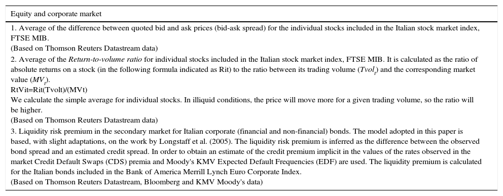
In Table 1, we provide a description of the variables used, grouped in sub-indices. Each sub-index is restricted to include at most three raw stress indicators, with the exception of the Italian government bond market, for which there are four indicators. Each raw indicator included in a sub-index should capture complementary information about the level of strains in the same market segment. The raw indicators in each sub-index should be perfectly correlated only under extreme liquidity situations, such as when market conditions become totally dysfunctional. In normal situations we should observe differentiation across the raw indicators in the same sub-index.
Description of the individual raw indicators grouped by sub-index.
| Equity and corporate market |
|---|
| 1. Average of the difference between quoted bid and ask prices (bid-ask spread) for the individual stocks included in the Italian stock market index, FTSE MIB. (Based on Thomson Reuters Datastream data) |
| 2. Average of the Return-to-volume ratio for individual stocks included in the Italian stock market index, FTSE MIB. It is calculated as the ratio of absolute returns on a stock (in the following formula indicated as Rit) to the ratio between its trading volume (Tvolt) and the corresponding market value (MVt). RtVit=Rit(Tvolt)/(MVt) We calculate the simple average for individual stocks. In illiquid conditions, the price will move more for a given trading volume, so the ratio will be higher. (Based on Thomson Reuters Datastream data) |
| 3. Liquidity risk premium in the secondary market for Italian corporate (financial and non-financial) bonds. The model adopted in this paper is based, with slight adaptations, on the work by Longstaff et al. (2005). The liquidity risk premium is inferred as the difference between the observed bond spread and an estimated credit spread. In order to obtain an estimate of the credit premium implicit in the values of the rates observed in the market Credit Default Swaps (CDS) premia and Moody's KMV Expected Default Frequencies (EDF) are used. The liquidity premium is calculated for the Italian bonds included in the Bank of America Merrill Lynch Euro Corporate Index. (Based on Thomson Reuters Datastream, Bloomberg and KMV Moody's data) |
| Italian government bond market |
|---|
| 1. Average of the difference between quoted bid and ask prices (bid-ask spread) on BTPs traded on the secondary market for government securities (MTS). (Based on Bank of Italy data) |
| 2. Average amount of the purchase and sale proposals that traders exhibit in the MTS book. (Based on Bank of Italy data) |
| 3. Amounts of Italian government bonds traded on the wholesale markets MTS and BondVision. (Based on Bank of Italy data) |
| 4. Volatility in the daily price of BTP future. It is calculated as the standard deviation of the logarithm of the daily change in the price of the BTP future. This indicator should take account of the effects of volatility shocks as an important driver of liquidity conditions in bond markets. (Based on Thomson Reuters data) |
| Money market |
|---|
| 1. The liquidity risk premium in the “unsecured” money market. The approach followed to infer the liquidity premium implicit in money market spreads is of an indirect type: first one infers the credit risk component in the spread between Euribor and the overnight indexed swap (OIS); then, the liquidity risk is gauged as the difference between the spread and the estimated credit risk component. Premia on CDS contracts on the banks in the Euribor panel form the dataset used in step 1 of this procedure. The model adopted is based, with some adaptations, on the work by Longstaff et al. (2005) for the corporate bonds. The data are 12-month CDS premia and 12-month money market rates. (Based on Thomson Reuters Datastream and Bloomberg data) |
| 2. Amounts traded on Italian unsecured and secured money markets e-MID, NewMIC, MTS/Repo (General Collateral, GC, and Special Repo, SR) (Based on Bank of Italy data) |
| 3. Volatility in the daily rate of interest of MTS/Repo GC with maturity Tom Next. It is calculated as the standard deviation of the logarithm of the daily change in the rate of interest. This indicator should take account of the effects of volatility shocks as an important driver of liquidity conditions in money markets. (Based on Bank of Italy data) |
Another issue of concern is related to the frequency of the indicator. High frequency indices give a more accurate picture of the level of stress in a given period. This may be a desirable result for policy makers; generally, systemic indicators that rely only on market data are of daily frequency while those that use both market and balance-sheet are of a lower frequency. In estimation of our indicator we use only on market data with a daily frequency.
4Methodology of the systemic liquidity risk indicatorThe methodology follows those commonly used for the indicators of systemic risk. It is divided into the following steps.
4.1Transformation of raw indicators by means of order statisticsThe individual raw liquidity risk indicators are standardized through a transformation based on their empirical cumulative distribution function (CDF) involving the computation of order statistics.
We prefer the CDF approach to “classic” standardization (i.e. by subtracting the sample mean from the raw indicator and dividing this difference by the sample standard deviation). Classic standardization, in fact, implicitly assumes variables to be normally distributed; but the fact that many raw indicators violate this assumption enhances the risk that the results obtained from the use of standardized variables are sensitive to outlier observations.
The CDF transformation projects raw indicators into variables which are unit-free and measured on an ordinal scale with range (0,1].
Let us denote one of the raw stress indicators as xt, where t goes from 1 to n, with n the total number of observations in the sample. The ordered sample is represented as (x[1], x[2], ..., x[n]) where x[1]≤x[2]≤...≤x[n]; we use [r] to denote the ranking number assigned to a particular realization of xt. The transformed indicator on the basis of the empirical CDF Fn(xt) assumes the following values:
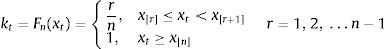
The empirical CDF Fn(x*) therefore measures the total number of observations xt not exceeding a particular value x* divided by the total number of observations in the sample. This transformation is applied recursively over expanding samples so that the transformed series is recalculated with one new observation added at a time:
for j=1, 2,…,N with N indicating the end of the full data sample.7Construction of sub-indices
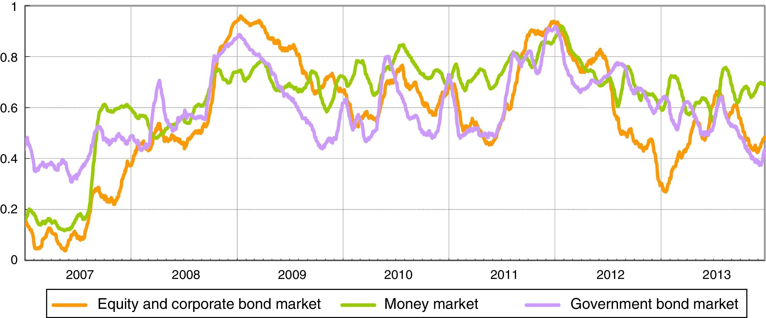
The set of ten homogenized raw liquidity risk indicators are grouped into three market categories (equity and corporate market, Italian government bond market and money market). Each raw indicator in a sub-index should capture complementary information about the level of strains in the same market segment. Each market category sub-index (si) are then calculated by taking arithmetic average (Fig. 1). This implies that each of the raw liquidity risk indicator is given equal weight in the sub-index.
.")
The three sub-indices reach the local maximum in the period after the Lehman default (end of 2008) and when sovereign debt tensions were most directly targeted on Italy and Spain (end of 2011).
4.2A portfolio based approach to the systemic liquidity risk indicatorIn order to aggregate the three sub-indices si into a systemic liquidity risk indicator, we follow the methodology suggested in Hollò et al. (2012), where concepts from portfolio theory are used. In portfolio theory, when highly correlated risky assets are aggregated, total portfolio risk increases as all assets tend to move together following the markets’ movement. By contrast, when the correlation between assets is low, diversifiable (non-systematic) risk is reduced and, as a consequence, the risk of total portfolio is also reduced. Total portfolio risk depends not only on the volatilities of the financial assets but also on their correlations (cross-correlations). In a way, as in portfolio theory, a high degree of correlation depicts a widespread liquidity risk in several segments of the market which, in turn, may lead to increased systemic risk.
As a result the systemic liquidity risk indicator (SLRI) for the Italian financial markets proposed in this paper puts relatively more weight on situations in which stress prevails in several market segments at the same time. It is computed according to:
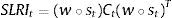
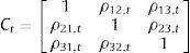
The systemic indicator's range of variation is (0,1], where 0 represents a situation with minimum systemic liquidity risk and 1 the maximum risk; w is the vector of (constant) equal sub-index weights; w∘st is the element by element multiplication of the vector of sub-index weights and the vector of sub-index values in time t (Hadamard-product); Ct is the matrix of time-varying cross-correlation coefficients ρiz,t between sub-indices i and z.
When all sub-indices are perfectly correlated, the SLRI would be equal to the square of the weighted average of the three sub-indices (i.e. the vector vt=w∘st); this would imply a situation in which all sub-indices stand either at historically low levels (low liquidity risk) or at historically high levels (high liquidity risk) at the same time. However, most of the time correlations are quite diverse and relatively lower than the case of perfect correlation, so that the SLRI assumes much lower levels than the weighted average composite indicator.
In order to calculate the SLRI, we need to estimate the time-varying cross-correlation matrix Ct. To do this, we implement a Multivariate GARCH (MGARCH) approach.8 In particular, we estimate the BEKK model (Baba et al., 1991; Engle and Kroner, 1995). The choice of BEKK appears optimal for the estimation of models of limited size (in this case n=3; Louzis and Vouldis, 2013): there are no convergence problems in the estimation and there is no need for restrictions on the parameters to ensure the positive definiteness of the conditional covariance matrix. Compared with classic methods of calculation of the correlation, the chosen method gives greater weight to more recent observations: the BEKK GARCH model allows us to capture abrupt changes in correlations and then identify events characterized by high systemic risk. In addition, contrary to the Moving Average metric like the exponentially weighted moving average (EWMA) this approach allow for fading gradually the effects of volatility shocks and avoiding arbitrariness in the choice of the decay factor (which provides a measure of the time after which each observation loses its influence on the estimate) and risks producing inconsistent parameter estimates.9
In its general form a BEKK(p,q,K) model is defined as:
where A is an n×n lower triangular matrix, Bki, Dkj are n×n parameter matrices, K specifies the generality of the process while p and q are the lags used (in our case p=q=K=1). The parameters of the BEKK model are estimated by maximizing the Gaussian likelihood function of the multivariate process. The most appealing property of the BEKK model is that it ensures the positive definiteness of the conditional covariance matrix, Ht, by using the product of the two lower triangular matrices as a constant term. Even if the BEKK model is relatively parsimonious compared with other MGARCH specifications, the number of parameters that have to be estimated is still high, even in the trivariate case. For this reason we impose a diagonal BEKK representation, where Bki and Dkj are restricted to be diagonal matrices.105Results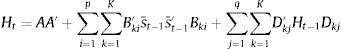
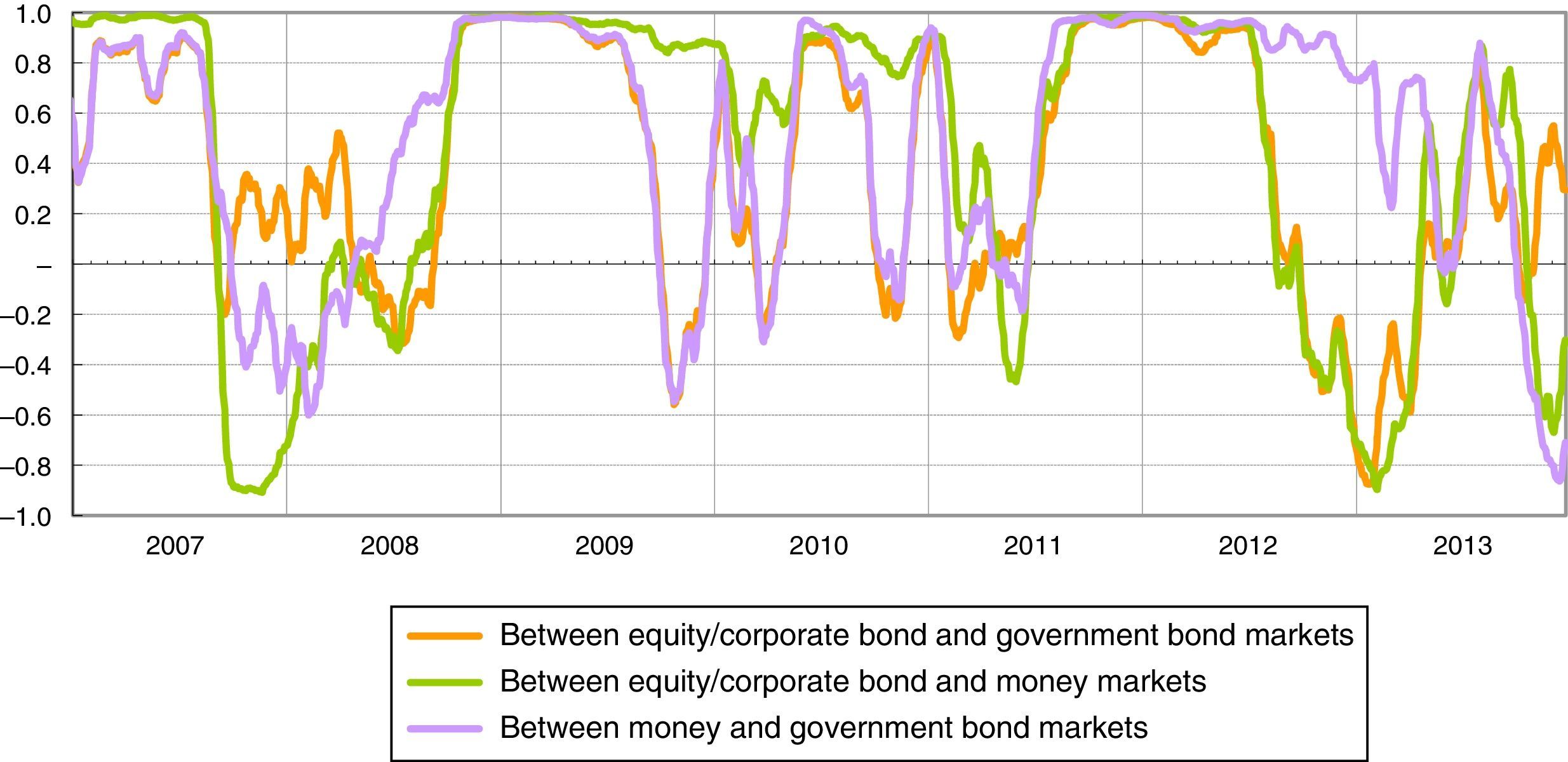
As pointed out in Section 4, an important feature of the methodology adopted is that it utilizes the time-varying cross-correlations between the sub-indices in order to capture and quantify systemic liquidity risk. Fig. 2 shows the correlations between the three sub-indices estimated with the diagonal BEKK model.
 (daily data; moving average at 20 days). (1) Cross-correlations between sub-indices are estimated with a diagonal GARCH BEKK.")
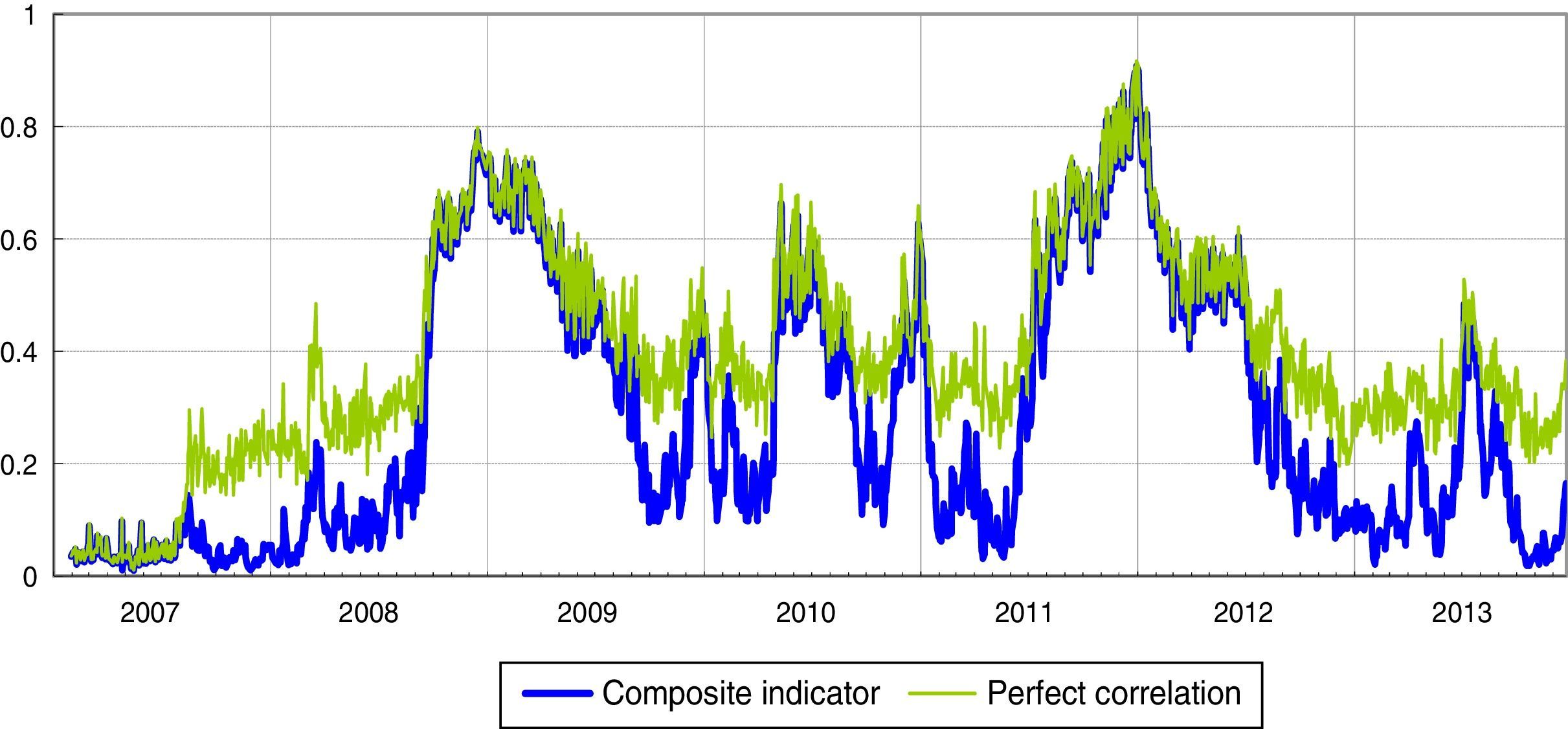
In the Italian financial markets there have been three periods in which the correlations between the sub-indices remained for prolonged periods at values almost equal to 1 (perfect correlation): (1) the period after the Lehman default; (2) the escalation of the Greek debt crisis and involvement in the sovereign debt crisis of other Eurozone countries, such as Ireland (April and November 2010); (3) the phase in which sovereign debt tensions primarily involved Italy and Spain (second half of 2011 and first half of 2012). These periods see the maximum values of the systemic liquidity risk indicator, respectively 0.8, 0.6 and 0.9 (Fig. 3).
 (daily data). (1) The green line represents the values of the indicator if sub-indices were perfectly correlated; in this case the indicator would be equal to the square of the weighted average of the three sub-indices. (For interpretation of the references to color in the text, the reader is referred to the web version of the article.)")
Systemic liquidity risk indicator: composite indicator versus hypothesis of perfect correlation (1) (daily data).
(1) The green line represents the values of the indicator if sub-indices were perfectly correlated; in this case the indicator would be equal to the square of the weighted average of the three sub-indices. (For interpretation of the references to color in the text, the reader is referred to the web version of the article.)
Whenever liquidity stress is extremely high (or extremely low) in all the market segments at the same time, all the cross-correlations increase considerably; when the time correlations are equal to one, the SLRI coincides with the indicator calculated assuming perfect correlation between markets (Fig. 3). It can therefore be said that the “perfect correlation” case overstates the level of liquidity stress in “normal times”, when correlations are relatively moderate, and introduces a bias in its information content in such circumstances. At the same time, we expect that during crisis periods the time-varying correlation-based indices will converge on the “perfect correlation” index as correlations converge to unity. However, indicators not incorporating the systemic nature of stress could provide misleading information regarding the “true levels” of strains in the financial system as a whole.
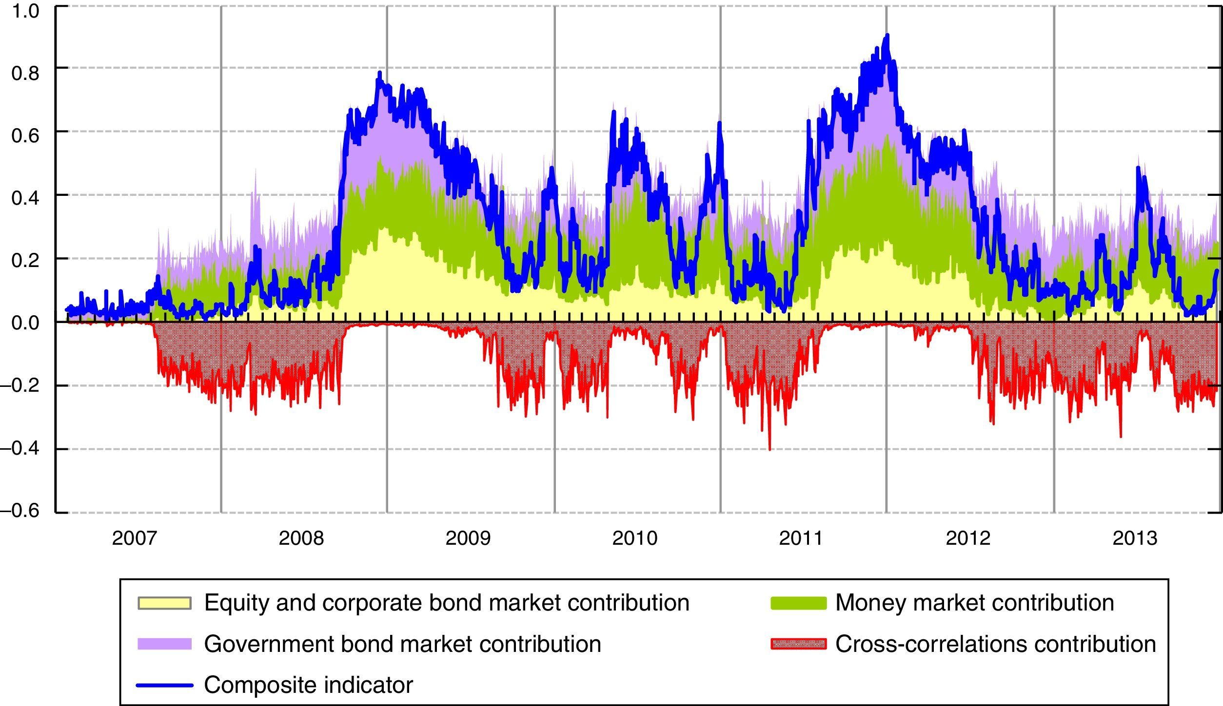
The comparison of the systemic indicator with the square of the weighted average of the sub-indices (“perfect correlation” index) also forms the basis for a decomposition of the SLRI into the contributions of each of the sub-indices and the overall contribution of all the cross-correlations; such a decomposition is very helpful for regular monitoring exercises (see Fig. 4).11
 (daily data). (1) Decomposition of the SLRI into the contributions of each sub-index (equity and corporate market, Italian government bond market and money market) and of all the cross-correlations jointly.")
During periods of major stress, such as the Lehman default in 2008 and the sovereign debt crisis in 2011, the cross-correlations increase, as represented graphically by the convergence of the red line of the contribution of cross-correlations to zero. In these two periods of stress, the tensions started in the money market and in the government bond market respectively. Nevertheless, we can observe quite a similar dynamic of the indicator because of the high cross-correlations, above all between the money and government bonds markets (see Fig. 2).
In a nutshell, Fig. 4 shows that the SLRI tends to react rapidly to strains in the Italian financial market, emphasizing the ability of the multivariate GARCH model to capture sudden changes in the correlations.
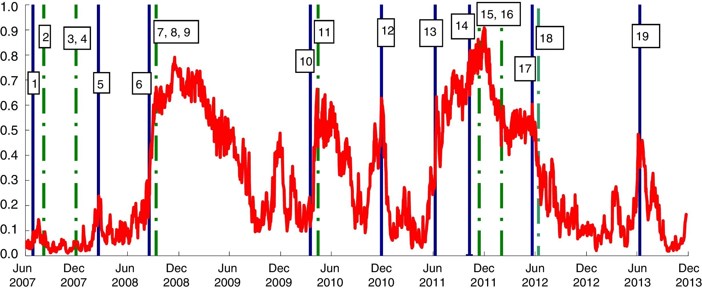
A visual analysis is carried out in Fig. 5. The liquidity risk indicator, as previously calculated, is shown together with vertical solid blue lines indicating the negative events which led to a rise in financial strains and dotted green vertical lines indicating the most important European Central Bank (ECB) actions. This evidence would suggest that the SLRI is a good indicator for measuring liquidity stress: it rose after negative events and fell after ECB actions.
![Systemic liquidity risk indicator and main financial “liquidity” events (1) (daily data; index number between 0 and 1). (1) The indicator's range of variation is (0,1], where 0 represents a situation with minimum systemic liquidity risk and 1 the maximum risk. 1: Start of the crisis; 2: Supplementary LTROs; 3, 4: US dollar liquidity-providing operations; fixed rate 2 week tender full allotment; 5: Bear Stearns default; 6: Lehman default; 7, 8, 9: Change to fixed rate tender with full allotment; narrowing of standing facilities corridor; expansion of list of eligible assets; 10: Concern over public finances in Greece; 11: Securities Market Program; 12: Ireland seeks financial support; 13: Renewed concern over public finances in a few euro-area countries; 14: Concerns more directly targeted on Italy and Spain; 15: 3 year LTRO and expansion of list of eligible assets; 16: Second 3year LTRO; 17: Spain requests financial assistance to recapitalize banking sector; 18: Draghi's speech “The ECB is ready to do whatever it takes” and OMT; 19: Tensions at end of the first half year and uncertainties about central counterparties's risk management policies. (For interpretation of the references to color in the text, the reader is referred to the web version of the article.)](https://static.elsevier.es/multimedia/21731268/0000001400000001/v1_201604060102/S2173126816000024/v1_201604060102/en/main.assets/gr5.jpeg?xkr=ue/ImdikoIMrsJoerZ+w997EogCnBdOOD93cPFbanNe1fKXdd/vmhD5L3AQCBc45J8X38KxykHquN95Qizi01AqMLo2cqp1gkL6g+wUmRJTq/VUZD1O/Pn2Wk8fKVLlHGZwHf7WEek7/HPTnudn/gQ+RIgd31+qRuzoofg10+7HDaIJQPkXmI0J0f4FZE1AdnaCZ4RuCuql+iMGq1e+k6nWw1XBi4bAMk8ZaGyCRRW9Tm0EgG3fXEPCV9AKrNwTGCllb33R6zlEpr1e/d/jzwBdM7s7YVbhPrQ6iVR3wvL9jMhAIYiHGl76kBiKJojucCrY/zHTrD8Rhi+MB26h3Iw== "Systemic liquidity risk indicator and main financial “liquidity” events (1) (daily data; index number between 0 and 1). (1) The indicator's range of variation is (0,1], where 0 represents a situation with minimum systemic liquidity risk and 1 the maximum risk. 1: Start of the crisis; 2: Supplementary LTROs; 3, 4: US dollar liquidity-providing operations; fixed rate 2 week tender full allotment; 5: Bear Stearns default; 6: Lehman default; 7, 8, 9: Change to fixed rate tender with full allotment; narrowing of standing facilities corridor; expansion of list of eligible assets; 10: Concern over public finances in Greece; 11: Securities Market Program; 12: Ireland seeks financial support; 13: Renewed concern over public finances in a few euro-area countries; 14: Concerns more directly targeted on Italy and Spain; 15: 3 year LTRO and expansion of list of eligible assets; 16: Second 3year LTRO; 17: Spain requests financial assistance to recapitalize banking sector; 18: Draghi's speech “The ECB is ready to do whatever it takes” and OMT; 19: Tensions at end of the first half year and uncertainties about central counterparties's risk management policies. (For interpretation of the references to color in the text, the reader is referred to the web version of the article.)")
Systemic liquidity risk indicator and main financial “liquidity” events (1) (daily data; index number between 0 and 1). (1) The indicator's range of variation is (0,1], where 0 represents a situation with minimum systemic liquidity risk and 1 the maximum risk.
1: Start of the crisis; 2: Supplementary LTROs; 3, 4: US dollar liquidity-providing operations; fixed rate 2 week tender full allotment; 5: Bear Stearns default; 6: Lehman default; 7, 8, 9: Change to fixed rate tender with full allotment; narrowing of standing facilities corridor; expansion of list of eligible assets; 10: Concern over public finances in Greece; 11: Securities Market Program; 12: Ireland seeks financial support; 13: Renewed concern over public finances in a few euro-area countries; 14: Concerns more directly targeted on Italy and Spain; 15: 3 year LTRO and expansion of list of eligible assets; 16: Second 3year LTRO; 17: Spain requests financial assistance to recapitalize banking sector; 18: Draghi's speech “The ECB is ready to do whatever it takes” and OMT; 19: Tensions at end of the first half year and uncertainties about central counterparties's risk management policies. (For interpretation of the references to color in the text, the reader is referred to the web version of the article.)
Before August 2007, the SLRI in the Italian financial markets was fairly stable, at around four to seven basis points, reflecting the fact that liquidity was flowing smoothly in the market segments considered.
The developments in the SLRI in the early months after the onset of the crisis (the autumn of 2007) mainly reflect the generalized surge in tensions in the money market that also affected Italian banks; in this phase the Italian government securities market and the equity market were not affected. The SLRI increased in the spring of 2008, with the Bear Stearns crisis, and accelerated after the Lehman default. In 2008, the Lehman collapse was the game changer in the liquidity market for its implications on the credit risk premium in the money market rates; this event was followed by an increase in the systemic risk in the financial markets. The central banks’ prompt response limited the negative effects. However, in the first months of 2009 pressure had already started to affect the government securities market as shown by the widening of the BTP/Bund spreads. This was mainly due not to the increase in sovereign risk but to the liquidation of government bond positions by some investors to cover losses reported in other markets or to obtain liquidity. As a consequence, bid/ask spreads widened and market liquidity declined.
The indicator fell dramatically after the ECB enacted unconventional loosening liquidity management policies. In the middle of 2009 it was very low compared with the estimated values after the Lehman default, which may be evidence in favor of the effectiveness of the various policies adopted by the ECB.
At the end of 2009 there began to be concern about the Greek public finances. In 2010, the pressure affected the government securities market more than the funding market, partly owing to an increase in risk aversion.
In the summer of 2011, stock markets fell due to fears of the spreading of the European sovereign debt crisis to Spain and Italy, as well as to concern about the slow economic growth of the United States and fear of its credit rating being downgraded. In November 2011 the increase in central counterparties’ margins in the repo market made the liquidity and funding problems even worse. This was a period of very low liquidity in the government bond market: moreover, ECB purchases were seen as an opportunity to sell and exit the market. The increase in sovereign risk and the widening of the BTP/Bund spread severely affected Italian banks, which suffered from the wrong way correlation (Italian banks/Italian collateral).
At the end of 2011 and in February 2012, the big take-up at the 3-year LTROs addressed the funding issue for Italian banks and led to an improvement in market sentiment. Italian banks regained access to the repo market (short tenors). In this period, the Italian repo market was much less sensitive to the sovereign tensions.
In 2013 the liquidity conditions in the Italian financial markets were satisfactory, although sensitive to the uncertainty that characterized some months of the year, particularly during the summer. In the summer the indicator increased rapidly, essentially reflecting temporary strains in the money market. In June and July interest rates in the Italian liquidity markets increased with respect to the euro area. The phenomenon should be tied to participants’ uncertainty concerning changes to central counterparties’ risk management policies, which were being finalized during the period. At the beginning of August these tensions were rapidly dispelled.
The increase in liquidity in the Italian repo market, mainly provided by some domestic institutions, helped to reduce the sensitivity of the Italian repo market to external factors (such as stricter regulation on liquidity, leverage ratios and central counterparties’ risk management policies). The liquidity conditions in the equity and corporate market also eased in the second half of 2013.
6Evaluation of the indicator6.1Identification of liquidity stress eventsAs shown in the previous paragraph, the SLRI seems to perform well in identifying periods of high financial stress by capturing the crisis periods accurately without exaggerating the level of stress during calm periods. Nonetheless a more formal approach is required in order to validate our findings.
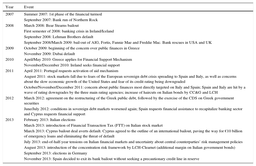
To this end, we conducted a survey among financial experts inside and outside the Bank of Italy to determine the most liquidity stressful events for the Italian financial markets. The aim of the survey was to rank historical events in terms of how stressful they were for the liquidity of the Italian financial markets. Thirty questionnaires were distributed. The questionnaire is shown in Appendix A. The list of events was drawn from a review of every Financial Stability Report of the Bank of England, the ECB and the Bank of Italy since 2005.12 Twenty-two events were identified.
The survey results established a qualitative benchmark with which to compare and evaluate the systemic liquidity risk indicator (Tables B.1–B.3 in Appendix B present the survey results and estimations). This approach was also used by Illing and Liu (2006) and Louzis and Vouldis (2013) to evaluate their financial stress indices, respectively, for Canada and Greece. The answers from the survey were used to construct a binary index of “severe” liquidity strains for the Italian financial markets. Systemic liquidity stress in the Italian financial markets was identified with events in which the average value of the answers exceeded the mean of the stress scale (2.5). The binary variable equals 1 if survey respondents felt Italian financial markets were under stress during the period in question, and 0 otherwise.
In order to gauge the performance of the indicator we estimate the following probit model:
where Φ is the cumulative distribution function of the standard normal distribution, yi is the binary index derived from the survey and xi comprises the constant and the systemic liquidity risk indicator.
Table B.2 shows the coefficient estimates, asymptotic standard errors, z-statistics and corresponding p-values. The coefficients have the expected sign and are statistically significant. Table B.2 also reports McFadden R-squared, which is the likelihood ratio index; as the name suggests, this is analogous to the R2 reported in linear regression models: it has the property that it always lies between zero and one. The SLRI provides a good fit for the liquidity crisis events identified by the financial market experts, measured by the McFadden R-squared (0.67).
Table B.3 reports a contingency table of correct and incorrect classification based on a specified prediction rule. In more detail, observations are classified by predicted probabilities according to whether they are above or below the specified cutoff value (which we set to the default value of 0.5).
Correct classifications are obtained when the predicted probability is less than or equal to the cutoff and the value of the binary index is equal to 0 (y=0), or when the predicted probability is greater than the cutoff and the value of the binary index is equal to 1 (y=1). In our estimation, 1611 of the y=0 observations and 467 of the y=1 observations are correctly classified by the estimated model. Overall, the estimated model correctly predicts 91.8 per cent of the observations (94.4 per cent of the y=0 observations and 83.7 per cent of the y=1 observations).
Lastly, we carry out two “goodness of fit” tests: Hosmer–Lemeshow (1989) and Andrews (1988). The chi square statistics are reported at the bottom of Table B.3. The p-value for both the tests is small, providing evidence of the goodness of the fit of our indicator.
A primary goal of the liquidity stress indicator is to provide a “snapshot” of the current degree of stress in the financial markets and to help policymakers in identifying strains in the financial markets that may be of serious concern; in this regard, identifying a threshold tied to a “severe” stress level is a challenge. The literature suggests several ways to tackle this problem. A relatively simple and widely used approach is to classify a stressful situation as “severe” if the indicator exceeds the threshold of one standard deviation above the median or mean (Illing and Liu, 2006).
One problem with this approach is how to identify “ex-ante” the number of standard deviations by which the indicator must exceed the historical mean or median to report a “severe” stress. In order to overcome this shortcoming, we apply an econometric approach which endogenously identifies periods of extreme stress in the Italian financial markets. We follow the methodology suggested in Hollò et al. (2012), where a regime classification based on an autoregressive Markov switching model is used. This approach is based on the assumption that the time series properties of the systemic indicator are state-dependent. This means that liquidity stress tends to display some intra-regime persistence, and that the transition between different states tends to occur stochastically.
We estimate several variants of a first-order autoregressive Markov-switching model for our indicator (xt), with two states (st), where all the coefficients are allowed to switch across states:
with residuals assumed to be standard, normal, independent and identically distributed (NID).
Our chosen model specification is an autoregressive process of order one (AR(1)) in which the intercept (α(st)), the slope coefficient (β(st)) and the residual variance (σ(st)) are allowed to switch across both the regimes. The choice is based on the Regime Classification Measure (RCM) proposed by Ang and Bekaert (2002) and refined by Baele (2005) for multiple regimes (see Table B.4 in Appendix B).
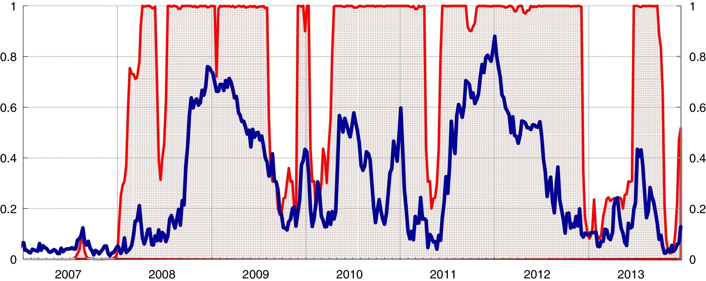
Tables B.5 and B.6 in Appendix B report for this model the coefficient estimates, standard errors, t-statistics, corresponding t-prob and the transition matrix probabilities. As shown in Fig. 6, the stress regime covers almost the entire period considered with different probability levels.
. (1) The blue line denotes the systemic liquidity risk indicator; the red line represents the smoothed probabilities of the stress regime (right-hand scale). Estimations based on weekly averages of daily data from January 2005 to December 2013. (For interpretation of the references to color in the text, the reader is referred to the web version of the article.)")
Systemic liquidity risk indicator and smoothed regime probabilities (1).
(1) The blue line denotes the systemic liquidity risk indicator; the red line represents the smoothed probabilities of the stress regime (right-hand scale). Estimations based on weekly averages of daily data from January 2005 to December 2013. (For interpretation of the references to color in the text, the reader is referred to the web version of the article.)
The ability of our indicator to capture abrupt changes in correlations and successfully identify events characterized by high systemic liquidity risk rests crucially on the adopted diagonal BEKK GARCH. In order to gauge the performance of our indicator and at the same time to provide a robustness check, we also estimate the indicator using two different specifications of the cross-correlations, respectively an exponentially weighted moving average (EWMA) model and a multivariate Dynamic Conditional Correlation (DCC) GARCH model, introduced by Engle (2002). We then evaluate the new values of the indicator on the basis of their ability to match the binary index constructed from the answers of the survey using the probit regression.
The results for all these stress indicators are presented in Table B.7. The fit of the indicator obtained from the EWMA specification, measured by the Mc-Fadden pseudo R-squared, is lower than that obtained using the BEKK GARCH; in the case of the DCC GARCH model, the Mc-Fadden measure deteriorated slightly but the p-value for the Hosmer–Lemeshow test is large while the value for the Andrews test statistic is small, producing mixed evidence of this model's ability to provide a good fit of the data. In sum, our indicator is robust to other specifications of the time-varying correlations. However the indicator calculated using the BEKK GARCH to estimate cross-correlations has the better fit.
Another desired property of a liquidity stress indicator is that the signals issued should be stable over time, so that it avoids the so-called “event reclassification” problem. As explained in Hollò et al. (2012), if at a particular point in time a stress indicator suggests that the prevailing level of stress is unusually high by historical standards, it would be desirable for the indicator to continue to classify this period as a stressful episode when new data are added to the sample for computing the indicator. This property is essential for regular use of the indicator as a practical tool for monitoring systemic liquidity risk.
In order to test this property we compare the values of the indicator when computed recursively with values obtained using the full data sample. We find that the two time series track each other very closely as evidenced by an average absolute value of 0.052 (standard deviation of 0.062) and a mean error of 0.048.
7ConclusionsThe financial crisis has illustrated the importance of timely and effective measures of systemic risk. Academics and financial authorities all around the globe are currently devoting much time and effort to developing tools and models which can be of help in measuring systemic risk. This paper contributes to this strand of the literature by introducing an indicator of systemic liquidity risk in the Italian financial markets.
The systemic nature of the indicator is based on the concept of correlation between market segments: the financial crisis has in fact shown that the relationships between the various market segments can amplify stress situations. In such a context the use of composite indicators built on simple aggregation (i.e. the mean) of individual measures produces an excessive simplification of reality with over- or underestimation of the impact of stress periods.
In order to overcome this shortcoming, we apply a portfolio theory based approach, suggested by Hollò et al. (2012), by modeling the time-varying cross-correlations between the sub-indices using a multivariate GARCH model. More specifically, we estimate the BEKK model, following Louzis and Vouldis (2013). This approach is able to capture abrupt changes in the correlation and makes it possible for the indicator to identify systemic liquidity events precisely.
In addition, the decomposition of the indicator into the contributions coming from each of the sub-indices and the overall contribution from the cross-correlations provides additional information on the behavior of individual markets and on how the cross-correlations work by amplifying or dampening stressful situations. This decomposition is very helpful for regular monitoring exercises.
Validation of the systemic liquidity risk indicator is based on a survey conducted among financial market experts, which was used to determine the most liquidity stressful events for the Italian financial markets. The systemic liquidity risk indicator was found to provide timely identification of crisis periods and the level of systemic liquidity stress in the Italian financial markets. The results also show that the systemic liquidity risk indicator does not exaggerate the level of stress during calm periods.
We have developed a systemic liquidity risk indicator for the Italian financial markets.
We would be grateful if you could provide us with your view regarding the impact of certain historical events on systemic liquidity conditions in the Italian financial markets.
The aim of this survey is to compare the level of liquidity stress, as measured by the systemic liquidity risk index, with your view of historical events.
We would like you to rank the following events in terms of how stressful they were for the liquidity of the Italian financial markets, where:
- •
1=not stressful
- •
2=somewhat stressful
- •
3=very stressful
- •
DK=don’t know
Please feel free to add comments in the margin:
| Year | Event |
|---|---|
| 2007 | Summer 2007: 1st phase of the financial turmoil |
| September 2007: Bank run of Northern Rock | |
| 2008 | March 2008: Bear Stearns bailout |
| First semester of 2008: banking crisis in Ireland/Iceland | |
| September 2008: Lehman Brothers default | |
| September 2008/March 2009: bail-out of AIG, Fortis, Fannie Mae and Freddie Mac. Bank rescues in USA and UK | |
| 2009 | October 2009: beginning of the concern over public finances in Greece |
| November 2009: Dubai default | |
| 2010 | April/May 2010: Greece applies for Financial Support Mechanism |
| November/December 2010: Ireland seeks financial support | |
| 2011 | April 2011: Portugal requests activation of aid mechanism |
| August 2011: stock markets fall due to fears of the European sovereign debt crisis spreading to Spain and Italy, as well as concerns about the slow economic growth of the United States and fear of its credit rating being downgraded | |
| October/November/December 2011: concern about public finances most directly targeted on Italy and Spain; Spain and Italy are hit by a wave of rating downgrades by the three main rating agencies; increase of haircuts on Italian bonds by CC&G and LCH | |
| 2012 | March 2012: agreement on the restructuring of the Greek public debt, followed by the exercise of the CDS on Greek government securities |
| June/July 2012: conditions in sovereign debt markets worsened again; Spain requests financial assistance to recapitalize banking sector and Cyprus requests financial support | |
| 2013 | February 2013: Italian elections |
| March 2013: introduction of Financial Transaction Tax (FTT) on Italian stock market | |
| March 2013: Cyprus bailout deal averts default. Cyprus agreed to the outline of an international bailout, paving the way for €10 billion of emergency loans and eliminating the threat of default | |
| July 2013: end-of-half-year tensions on Italian financial markets and uncertainty about central counterparties’ risk management policies | |
| August 2013: introduction of the concentration risk framework by LCH-Clearnet (additional margin on Italian government bonds) | |
| September 2013: elections in Germany | |
| November 2013: Spain decided to exit its bank bailout without seeking a precautionary credit line in reserve |
The following are the supplementary data to this article:
Any views expressed in this paper are the authors’ and do not necessarily represent those of the Bank of Italy.
See IMF (2009) and Bisias et al. (2012) for surveys.
See Chordia et al. (2000), who study market liquidity, and Chordia et al. (2001), who analyze the correlation of liquidity measures between markets.
Given the considerable computational burden resulting from the recursive estimation, in the paper we present results which are estimated on the entire sample.
See Alexander (2008) and Andersen et al. (2003) for a description of Multivariate GARCH models.
The sum of the contributions from each sub-index, by ignoring their cross-correlations, is represented in the figure by the upper border of the purple area and is thus equivalent to the weighted average of the three sub-indices. The difference between this “average” SLRI and the SLRI proper thus reflects the impact of the cross-correlations and is plotted in the figure as the area below the zero line. See Hollò et al. (2012).


- Download PDF
- Bibliography
- Additional material