


Using the Efficient Method of Moments we estimate a continuous time diffusion for the stochastic volatility of some international stock market indices that allows for possible jumps in returns. These jumps are needed for a sensible characterization of the dynamics of the distribution of returns, even under stochastic volatility. Although the stochastic volatility model with jumps in returns tends to exaggerate the negative skewness relative to the sample moments, the inclusion of jumps strongly improves the ability of the model to replicate sample kurtosis. This contrasts with the failure of the pure stochastic volatility model in generating high enough kurtosis. Our results extend the limited available evidence from the U.S. market to several European stock market indices.
Financial economists achieved unprecedented success over the last thirty years using simple diffusion models to approximate the stochastic process for returns on financial assets. The so-called volatility smiles and smirks computed using the volatility implied by the Black-Scholes model reveal, however, that a simple geometric Brownian motion process misses some important features of the data. This limitation is very relevant, since empirical evidence suggests that practical financial decision making based on the continuous time setting will be satisfactory only if it builds upon reasonable specifications of the underlying asset price processes. In other words, the actual distribution of the underlying asset implied by the data must be consistent with the distribution assumed by the theoretical model.
High frequency return data displays excess kurtosis (fat tailed distributions), skewness, and volatility clustering. Capturing these essential characteristics with a tractable parsimonious parametric model is difficult, but it is widely accepted that incorporating stochastic volatility or jumps into continuous time diffusion processes can help explain these main statistical characteristics of observed financial returns. Unfortunately, existing results for U.S. data have so far been inconclusive or contradictory, and most studies fail to produce a satisfactory fit to the underlying asset return dynamics.
As initial papers in a rapidly increasing literature, Andersen et al. (2002) estimated models with jumps in prices and stochastic volatility, and Chernov et al. (2003) and Eraker et al. (2003), added jumps in volatility to that specification. All of them found strong evidence for stochastic volatility and jumps in prices, but they disagreed over the presence and importance of jumps in volatility, and over the convenience to allow for state-dependent arrival of jumps. The available evidence for U.S. data consistently find that allowing for jumps in returns helps matching the observed distribution of returns with relatively smooth volatility. If the process does not allow for jumps, then replication of sample kurtosis requires a higher volatility of the stochastic variance process, to compensate for the absence of jumps. In addition to its kurtosis, the jump-diffusion process allows for two sources of skewness: a nonzero (usually negative) mean jump and the negative correlation between the shocks in returns and volatility. Both features help the model to match the negative skewness observed in sample moments. However, it should be pointed out that stochastic volatility is also important. If we do not allow for stochastic volatility, the estimated frequency of jumps is extraordinarily large, to compensate for the misspecification in the variance process.
The goal of this paper is to compare the appropriateness of a diffusion stochastic volatility model with jumps in returns to approximate the S&P 500 return dynamics as well as some European indices: DAX 30, IBEX 35 and CAC 40. We are particularly interested in analyzing whether the estimates can reproduce important aspects of the distribution of returns like third and fourth order moments. It is surprising the lack of evidence available regarding the behavior of continuous-time models for European return indices in spite of their relevance for asset allocation or for pricing derivatives. This paper fills that gap.
Until recently, a major obstacle for testing continuous-time models of equity returns was the lack of feasible techniques for estimating and drawing inference on general continuous time models using discrete observations. The main difficulty is that closed form expressions for the discrete transition density generally are not available, especially in the presence of unobserved and serially correlated state variables, as it is the case in stochastic volatility models. One way to respond to this challenge is the Simulated Method of Moments (SMM hereafter) of Duffie and Singleton (1993) that matches sample moments with simulated moments computed from a long time series obtained from the assumed data generating mechanism, also known as the structural model. Together with the Markov Chain Monte Carlo Bayesian estimator (MCMC), the SMM method is increasingly used because of their tractability and potential econometric efficiency, especially in situations with latent variables or under complex specifications of the jump component.
We adopt a variant of the SMM known as the Efficient Method of Moments (EMM hereafter), proposed by Bansal et al. (1993, 1995) and developed by Gallant and Tauchen (1996). EMM is a simulation based moment matching procedure with certain advantages. The moments to be matched are the scores of an auxiliary model called the score generator. As shown by Tauchen (1997) and Gallant and Long (1997), if the score generator is able to approximate the probability distribution of return data reasonably well, then estimates of the parameters of the structural model are as efficient as maximum likelihood estimates.
The paper is organized as follows: Section 2 presents the continuous time models for stock returns. Section 3 describes the details of the EMM methodology. Empirical results are given in Section 4, and Section 5 contains the concluding remarks.
2Model specification2.1Stochastic volatility (SV) modelA natural extension of the diffusion models widely applied in the asset pricing literature incorporates stochastic volatility to accommodate the clusters of volatility usually observed in stock market returns.1 This feature can explain broad general characteristics of actual return data, such as leptokurtosis and persistent volatility, and it is potentially useful in pricing derivatives. Hull and White (1987), Melino and Turnbull (1990), and Wiggins (1987) generalize the traditional geometric Brownian motion specification underlying the Black-Scholes expression by allowing for stochastic volatility to price equity and currency options. In a key contribution to literature, Heston (1993) allows for correlation between the Brownian motions in the mean and the variance equations, obtaining closed form expressions for option valuation using the Fourier inverse transform of the conditional characteristic function. In particular, Heston (1993) allows for a volatility risk premium that is proportional to the square root of the stochastic variance. This is the specification we employ in this research.
Let St be the price at t of a stock market index, with st=ln St. The square root stochastic volatility model (SV) is given by,
where the variance V follows a diffusion process with mean reversion in levels:with W1, W2 being correlated standard Brownian motions, corr(dW1,t,dW2,t)=ρdt.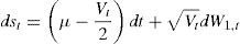

Stochastic volatility induces an excess of kurtosis through the values of α, β and η. The parameter β measures the speed at which the process reverts to the long-term variance (α/β), and it captures the persistence in variance. If the variance is highly volatile, i.e., if η is large, the probability of observing large shocks in returns will increase, and the tails of the distribution will be thicker. The skewness usually observed in returns can be captured through a negative correlation between shocks in variance and in returns, ρ<0. That way, volatility will increase when prices go down, thereby increasing the likelihood of large negative returns.
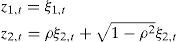
We obtain the first-order Euler discretization of our structural continuous-time diffusion process,
where M is the number of subperiods considered each day, Δ=1/M, and ξ1,t,ξ2,t,i.i.d.∼N(0,1), corr(ξ1,t,ξ2,t)=0. Hence, (z1,t,z2,t)∼N(0,1) with correlation ρ.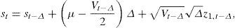

This discrete-time representation will provide us with simulated time series for returns that will be used to estimate the parameter vector with a better match to the score vector of an auxiliary model fitted to the data. We start by simulating time series data for ξ1t, ξ2t, from their respective probability distributions. From them, we get time series realizations for z1t, z2t. We take as initial price: S0=100, and a starting stochastic volatility Vt equal to its unconditional mean, V0=α/β. Once we have observations for logged prices, we compute log returns each subperiod rt=st−st−Δ, add them up over the M daily subperiods, to obtain daily returns. In our simulations, we take M=10 subperiods per day.2
2.2Stochastic volatility model with jumps (SVJ)It has recently become evident that success in fitting the dynamics of conditional volatility does not guarantee a good fit of the high conditional kurtosis in returns that is observed in many financial assets.3
We therefore add a jump component to the previous specification,
where the variance process V follows a mean-reverting diffusion as (2). We denote by qt a Poisson process, uncorrelated with W1 and W2, with a constant jump intensity λ, so that Pr(dqt=1)=λdt. The size of a jump at time t, if it occurs, is denoted by kt. We follow Andersen et al. (2002) in assuming that the size of the jump process follows a Normal distribution: ln(1+kt)≈N(−0.5δ2,δ2). This way, we are assuming that the mean jump in prices is zero.4 Even though we lose the contribution of k¯ to a negative skewness, imposing k¯=0 leads to a mean jump size in returns of −0.5δ2, implying more high negative jumps than positive ones, again contributing to negative skewness.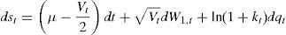
Hence, the model we simulate is:
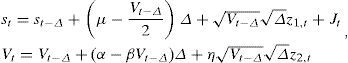
To simulate, we proceed as in the model without jumps in the previous section, simulating a time series data for ln(1+kt) from its probability distribution. The jump component is obtained as:
where I denotes an indicator function that takes a value of 1 when the condition in brackets holds, and it is equal to zero otherwise. Jumps are added to each return when they happen to materialize. In principle, it is possible that more than one jump occurs in a single day, although the probability of such event is very small. Finally, we aggregate log returns over each market day.3EMM estimation methodology
The first step of the estimation procedure consists of computing the quasi-maximum likelihood (QML) estimate of the parameters in the conditional density of index returns, which is approximated by a semi-nonparametric (SNP) density function.5 The approximation considers an auxiliary model made up by a constant plus a MA(1) innovation for returns, and a GARCH(1,1) representation for ht, the conditional variance of the innovations,6
A non-parametric term, made up by a number of Hermite polynomials, is included in the approximation to the density function to accommodate the non-Gaussian features of the return process. Since daily returns have negligible mean, we set π=0 in estimation. Furthermore, we follow Andersen et al. (2002) in prefiltering the return data using a simple MA(1) model and rescaling the residuals to match the sample mean and variance of the original data set. The obtained series is treated as the observed return process. This is justified by the fact that the inference on the volatility process is largely unaffected by the short-run mean dynamics, and it simplifies the estimation process.
Hence, the SNP density fK takes the form
where rt, xt=(rt−1,...,rt−L), t=1,…,∞ are the random variables corresponding to the index return process and lagged returns, ϕ(⋅) denotes the standard normal density, ν is a small constant,7zt=rt/ht is the standardized process of daily returns, and the polynomial PK(z,x) is a Kzth order polynomial in z, PK(z,x)=∑i=0KzaiHei¯(z), a0=1, where Hei¯(z) is the orthogonal Hermite polynomial of degree i.8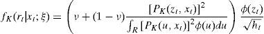
With this normalization, the fK density is interpreted as an expansion whose leading term is the Normal density ϕ(⋅), while higher order terms adapt to minor deviations from the Normal. In fact, the main task of the nonparametric polynomial expansion in the conditional density is to capture any excess kurtosis in the return process and any skewness which has not already been accommodated by the leading term.
The parameters ξ=(γ0,γ1,ϑ1,a1,a2,…,aKz) of the auxiliary model are estimated by QML by solving the problem:
where r˜t,x˜t=(r˜t−1,…,r˜t−L),t=1,…,n are the observed data, and n denotes the sample size.
The second step of the estimation procedure consists of estimating the parameters of the structural model, the diffusion process, so as to capture the main statistical characteristics in the data, as reflected in the mathematical expectation of the QML gradient, m(ψ,ξ˜)=∫((∂ln fK(r|x;ξ˜))/∂ξ)dP(r|x;ψ). The sample moment, mN(ψ,ξ˜)=(1/N)∑t=1N(∂ ln fK(rˆt(ψ)|xˆt(ψ);ξ˜))/∂ξ substitutes in estimation for the mathematical expectation m(ψ,ξ˜), where {rˆt(ψ),xˆt(ψ)}t=1N denote a sample simulated from the structural model using the parameter vector ψ.
The EMM estimator of ψ is then obtained following a GMM approach, minimizing the quadratic form,
for an appropriate weighting matrix I˜−1. Minimization of the quadratic form needs to be implemented by simulation, since it is not feasible to compute the analytical expression for the gradient of the likelihood under the structural model.
The expectation of the score function of the auxiliary model, mN(ψ,ξ˜), is evaluated by Monte Carlo integration at the quasi-maximum likelihood estimate of the parameter vector ξ˜ in the auxiliary model, and the weighting matrix I˜−1 is a consistent estimate of the asymptotic covariance matrix of the density fK, which is estimated from the outer product of the gradient9:
We use N=10000. N must be large enough so that the Monte Carlo simulation error in the gradient of the log likelihood can be considered to be negligible. The problem is that we would literally need millions of observations so that the error is insignificant as discussed by Andersen and Lund (1997). We also use the variance reduction technique of antithetic variables suggested by Geweke (1996), which is quite effective as shown, among others, by Andersen and Lund (1997) in reducing the discretization bias. The idea is to average two estimations of the integral m(ψ,ξ˜)=∫((∂ ln fK(r|x;ξ˜))/∂ξ)dP(r|x;ψ) which are supposed to be negatively correlated. We first compute the gradient of the likelihood using random variables (z1,t,z2,t), mN(z1t,z2t)(ψ,ξ˜). The second estimation, mN(−z1t,−z2t)(ψ,ξ˜), is computed using the same random numbers with the opposite sign: (−z1,t,−z2,t). Finally, mN(ψ,ξ˜)=(1/2)[mN(z1t,z2t)(ψ,ξ˜)+mN(−z1t,−z2t)(ψ,ξ˜)].
We take N1=N2=1000 and simulate two antithetic samples of (N+N2)×M+N1=(10 000+1000)×10+1000 for log-returns {rˆt(ψ)}t=1N using an Euler approximation (of order one) from the continuous time model at time intervals of 1/10 of a day. We discard the first N1 simulated values of st to eliminate the effect of the initial conditions. Then, a sequence of 11000 daily returns is obtained by summing the elements of the simulated sample in groups of 10. To reduce the potential bias that might be produced by the random number generator we discard the first N2 observations of those returns. That way, we end up with 10000 daily returns. In estimation, we maintain fixed the realization of the two fundamental N(0,1) innovations. The realizations for (z1,t,z2,t) will nevertheless change, because the parameter vector is changing in each iteration of the algorithm.
In our choice of auxiliary model, there are 4 parameters in the parametric component of the auxiliary model and 6 coefficients in the Hermite polynomials, for a total of 10 parameters. On the other hand, the structural model has 5 parameters if we do not include jumps in returns, and 7 parameters if jumps are considered. Hence, the identification condition dim(ψ)≤dim(ξ) holds, and we can proceed to implement the global specification test.
Once we get estimates for the parameters in the auxiliary model, the minimized value of the objective function follows a Chi-squared distribution:
where f(ψˆ,ξ˜) is the numerical value of the objective function at the final estimate and we can implement a global specification test by comparing the statistic above with the appropriate percentile of a Chi-square distribution with dim(ξ)−dim(ψ) degrees of freedom, which is either 5 or 3, depending on whether we consider the basic stochastic volatility model or the specification with jumps in returns. We can also compute t-ratios for the individual elements of the score, by dividing their estimates by their standard errors, tˆ=mN(ψˆ,ξ˜)/diag(S) where S=(1/n)(I˜−Mψ(M′ψI˜−1Mψ)−1M′ψ) and Mψ=∂mN(ψˆ,ξ˜)/∂ψ, which must be computed by numerical differentiation. Individual significance tests for these components can throw some light on the appropriateness of the auxiliary ability of the model to capture the main statistical features of the structural model, or some features of the data that the model is unable to approximate correctly.4Empirical results
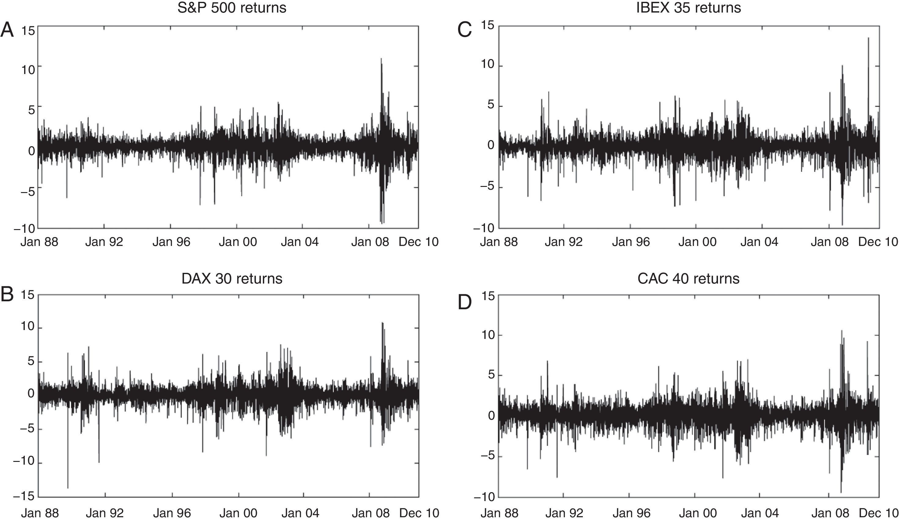
We have daily data from January 3, 1988 to December 30, 2010, with 5799 sample observations data for S&P 500, 5915 observations for DAX 30, 5764 for IBEX 35 and 5806 observations for CAC 40 (Fig. 1). Index returns display important kurtosis (between 8 and 12) and negative skewness (between −0.03 and −0.26), so the data generating process must be able to produce these same statistical characteristics in simulated returns.
, DAX 30 (Panel B), IBEX 35 (Panel C) and CAC 40 (Panel D), have 5799, 5915, 5764 and 5806 observations, respectively.")
S&P 500, DAX 30, IBEX 35 and CAC 40 daily rate of return. All data are expressed on a daily basis percentage form, from January 4, 1988 to December 30, 2010. Daily rates of return of the S&P 500 (Panel A), DAX 30 (Panel B), IBEX 35 (Panel C) and CAC 40 (Panel D), have 5799, 5915, 5764 and 5806 observations, respectively.
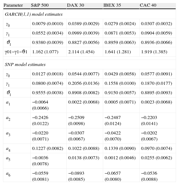
For each stock market index, we start by estimating the SNP specification of the auxiliary model, with parameter estimates and standard errors shown in Table 1. We also present estimates for the pure GARCH(1,1) for comparison. As expected, volatility displays high persistence in the four indices, and the long term GARCH volatility is close to the sample standard deviation, reflecting the fact that the model specification allows for almost no predictability of daily returns.10 By and large, estimated parameters in the SNP density are statistically significant.
SNP model.
| Parameter | S&P 500 | DAX 30 | IBEX 35 | CAC 40 |
| GARCH(1,1) model estimates | ||||
| γ0 | 0.0079 (0.0010) | 0.0389 (0.0029) | 0.0279 (0.0024) | 0.0307 (0.0032) |
| γ1 | 0.0552 (0.0034) | 0.0989 (0.0039) | 0.0871 (0.0053) | 0.0904 (0.0059) |
| ϑ1 | 0.9380 (0.0039) | 0.8827 (0.0056) | 0.8959 (0.0063) | 0.8936 (0.0066) |
| γ01−γ1−ϑ1 | 1.162 (1.077) | 2.114 (1.454) | 1.641 (1.281) | 1.919 (1.385) |
| SNP model estimates | ||||
| γ0 | 0.0127 (0.0018) | 0.0544 (0.0077) | 0.0429 (0.0058) | 0.0577 (0.0091) |
| γ1 | 0.0800 (0.0074) | 0.2056 (0.0136) | 0.1558 (0.0100) | 0.1870 (0.0177) |
| ϑ1 | 0.9555 (0.0038) | 0.8908 (0.0082) | 0.9150 (0.0057) | 0.8895 (0.0093) |
| a1 | −0.0064 (0.0066) | 0.0022 (0.0068) | 0.0005 (0.0071) | 0.0023 (0.0068) |
| a2 | −0.2426 (0.0122) | −0.2509 (0.0098) | −0.2487 (0.0124) | −0.2203 (0.0141) |
| a3 | −0.0220 (0.0071) | −0.0307 (0.0067) | −0.0422 (0.0070) | −0.0202 (0.0067) |
| a4 | 0.1227 (0.0082) | 0.1022 (0.0088) | 0.1339 (0.0090) | 0.0970 (0.0074) |
| a5 | −0.0036 (0.0078) | 0.0138 (0.0073) | 0.0012 (0.0046) | 0.0255 (0.0062) |
| a6 | −0.0559 (0.0081) | −0.0893 (0.0085) | −0.0657 (0.0080) | −0.0536 (0.0088) |
The reported results are expressed in percentage form. They are obtained from daily returns, filtered using a MA(1). The SNP model is: fK(rt|xt;ξ)=ν+(1−ν)[PK(zt,xt)]2/∫R[PK(u,xt)]2ϕ(u)du(φ(zt)/ht), where ν=0.01, φ(⋅) is the standard normal density, zt=rt/ht, ht=γ0+γ1rt−12+ϑ1ht−1∼GARCH(1,1) and PK(z,x)=∑i=0KzaiHei¯(z), a0=1.
Standard errors are given in parenthesis, except for the long-term variance γ0/(1−γ1−ϑ1), where we show in brackets the long-term GARCH standard deviation.
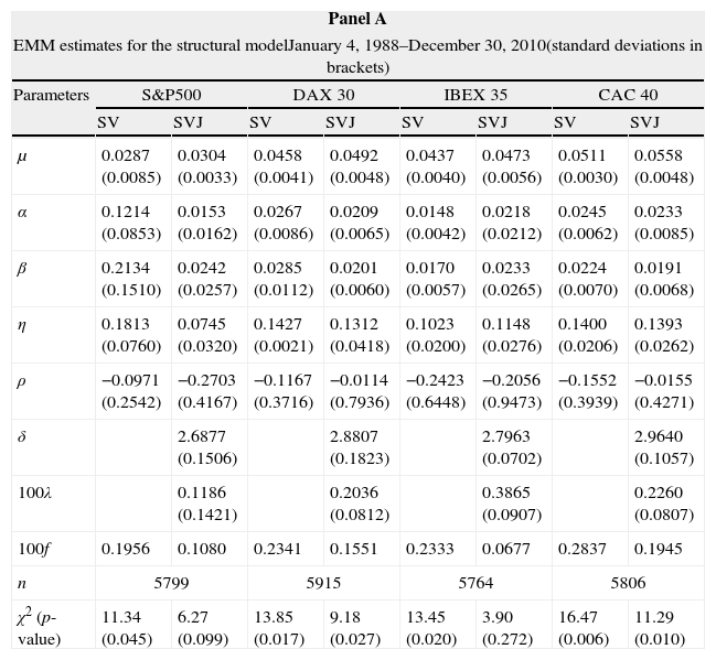
Once we have numerical estimates for the auxiliary model, we can proceed to estimating the parameters in the two structural models, SV and SVJ. Table 2 displays results in daily percent terms for each index and each structural model. Panel A shows parameter values and the minimized value of the objective function, together with the corresponding Chi-square statistic, while Panel B shows values for the t-ratios for the score vector, together with their p-values. Panel C compare sample moments to those obtained from the simulated time series from the estimated structural model.
EMM results of the stochastic volatility model (SV) and stochastic volatility model with jumps in returns (SVJ).
| Panel A | ||||||||
| EMM estimates for the structural modelJanuary 4, 1988–December 30, 2010(standard deviations in brackets) | ||||||||
| Parameters | S&P500 | DAX 30 | IBEX 35 | CAC 40 | ||||
| SV | SVJ | SV | SVJ | SV | SVJ | SV | SVJ | |
| μ | 0.0287 (0.0085) | 0.0304 (0.0033) | 0.0458 (0.0041) | 0.0492 (0.0048) | 0.0437 (0.0040) | 0.0473 (0.0056) | 0.0511 (0.0030) | 0.0558 (0.0048) |
| α | 0.1214 (0.0853) | 0.0153 (0.0162) | 0.0267 (0.0086) | 0.0209 (0.0065) | 0.0148 (0.0042) | 0.0218 (0.0212) | 0.0245 (0.0062) | 0.0233 (0.0085) |
| β | 0.2134 (0.1510) | 0.0242 (0.0257) | 0.0285 (0.0112) | 0.0201 (0.0060) | 0.0170 (0.0057) | 0.0233 (0.0265) | 0.0224 (0.0070) | 0.0191 (0.0068) |
| η | 0.1813 (0.0760) | 0.0745 (0.0320) | 0.1427 (0.0021) | 0.1312 (0.0418) | 0.1023 (0.0200) | 0.1148 (0.0276) | 0.1400 (0.0206) | 0.1393 (0.0262) |
| ρ | −0.0971 (0.2542) | −0.2703 (0.4167) | −0.1167 (0.3716) | −0.0114 (0.7936) | −0.2423 (0.6448) | −0.2056 (0.9473) | −0.1552 (0.3939) | −0.0155 (0.4271) |
| δ | 2.6877 (0.1506) | 2.8807 (0.1823) | 2.7963 (0.0702) | 2.9640 (0.1057) | ||||
| 100λ | 0.1186 (0.1421) | 0.2036 (0.0812) | 0.3865 (0.0907) | 0.2260 (0.0807) | ||||
| 100f | 0.1956 | 0.1080 | 0.2341 | 0.1551 | 0.2333 | 0.0677 | 0.2837 | 0.1945 |
| n | 5799 | 5915 | 5764 | 5806 | ||||
| χ2 (p-value) | 11.34 (0.045) | 6.27 (0.099) | 13.85 (0.017) | 9.18 (0.027) | 13.45 (0.020) | 3.90 (0.272) | 16.47 (0.006) | 11.29 (0.010) |
| Panel B | ||||||||
| t-ratios for the elements of the score vector(p-values in brackets)Sample: January 4, 1988–December 30, 2010 | ||||||||
| Parameter | S&P 500 | DAX 30 | IBEX 35 | CAC 40 | ||||
| SV | SVJ | SV | SVJ | SV | SVJ | SV | SVJ | |
| γ0 | −0.285 (0.79) | 0.281 (0.81) | −1.937 (0.25) | −0.236 (0.84) | −1.365 (0.24) | 1.689 (0.23) | −3.455 (0.03) | 6.307 (0.98) |
| γ1 | −0.546 (0.61) | −1.271 (0.33) | −3.035 (0.73) | −2.493 (0.13) | −1.288 (0.27) | −1.712 (0.23) | −4.069 (0.02) | −7.110 (0.64) |
| ϑ1 | −0.556 (0.61) | −1.867 (0.20) | −2.695 (0.56) | −1.445 (0.13) | −1.521 (0.20) | −2.455 (0.13) | −3.578 (0.02) | −6.775 (0.69) |
| a1 | 1.792 (0.15) | −1.540 (0.26) | 2.404 (0.02) | −2.153 (0.16) | 1.690 (0.17) | −1.696 (0.23) | 7.076 (0.00) | −4.711 (0.15) |
| a2 | −3.265 (0.03) | −4.686 (0.04) | −4.282 (0.23) | −4.880 (0.04) | −2.997 (0.04) | −57.657 (0.00) | −3.681 (0.02) | −4.456 (0.45) |
| a3 | 0.321 (0.76) | 0.377 (0.74) | 0.720 (0.47) | −0.442 (0.70) | 0.394 (0.71) | 0.285 (0.80) | −3.264 (0.03) | 0.496 (0.83) |
| a4 | −0.666 (0.54) | −7.125 (0.02) | −2.159 (0.57) | −1.149 (0.37) | −0.877 (0.43) | −1.919 (0.19) | 0.594 (0.58) | −3.313 (0.67) |
| a5 | 0.624 (0.57) | 6.434 (0.02) | 3.624 (0.40) | 2.144 (0.17) | 0.888 (0.42) | 1.386 (030) | 1.570 (0.19) | 4.347 (0.63) |
| a6 | 1.163 (0.31) | −0.456 (0.69) | 1.064 (0.12) | 3.285 (0.08) | 0.241 (0.82) | −0.235 (0.84) | 0.446 (0.68) | −0.925 (0.93) |
| Panel C | ||||||
| Mean | Std. Dev. | Skewness | Kurtosis | Minimum | Maximum | |
| S&P 500 | ||||||
| Sample | 0.027 | 1.153 | −0.264 | 12.035 | −9.470 | 10.960 |
| SV | 0.013 | 0.758 | −0.209 | 3.460 | −3.690 | 3.100 |
| SVJ | −0.001 | 0.816 | −0.528 | 5.570 | −7.530 | 3.570 |
| DAX 30 | ||||||
| Sample | 0.025 | 1.438 | −0.243 | 9.482 | −13.710 | 10.800 |
| SV | 0.005 | 1.007 | −0.607 | 4.540 | −6.440 | 4.090 |
| SVJ | −0.018 | 1.095 | −1.023 | 8.620 | −14.470 | 4.270 |
| IBEX 35 | ||||||
| Sample | 0.029 | 1.335 | −0.163 | 8.141 | −9.580 | 10.120 |
| SV | 0.020 | 0.967 | −0.613 | 4.570 | −6.310 | 4.080 |
| SVJ | 0.012 | 1.040 | −1.070 | 9.550 | −13.990 | 4.050 |
| CAC 40 | ||||||
| Sample | 0.023 | 1.388 | −0.035 | 7.911 | −9.471 | 10.595 |
| SV | −0.016 | 1.099 | −0.690 | 4.720 | −7.410 | 4.390 |
| SVJ | −0.042 | 1.195 | −1.021 | 7.970 | −14.980 | 4.530 |
Panel A: EMM estimates: Estimates are expressed in percentage form on a daily basis. The rates of return of the S&P 500, DAX 30, IBEX 35 and CAC 40, correspond to the sample period from January 4, 1988 to December 30, 2010. Returns of the stock market indices have 5799, 5915, 5764 and 5806 observations, respectively. The estimates refer to the following models:
SV: dst=(μ−(Vt/2))dt+VtdW1,t, dVt=(α−βVt)dt+ηVtdW2,t.
SVJ: dst=(μ−(Vt/2))dt+VtdW1,t+ln(1+kt)dqt, dVt=(α−βVt)dt+ηVtdW2,t, ln(1+kt)≈N(−0.5δ2,δ2), corr(dW1,t,dW2,t)=ρdt, Pr(dqt=1)=λdt.
Panel B: EMM diagnosis: t-ratios of the elements of the score vector, which are given by tˆ=mN(ψˆ,ξ˜)/diagS where S=(1/n)(I˜−Mψ(M′ψI˜−1Mψ)−1M′ψ), Mψ=∂mN(ψˆ,ξ˜)/∂ψ. They correspond to the auxiliary model: fK(rt|xt;ξ)=ν+(1−ν)[PK(zt,xt)]/∫R[PK(u,xt)]2ϕ(u)du(φ(zt)/ht), where ν=0.01, φ(⋅) is the standard normal density, zt=rt/ht, ht=γ0+γ1rt−12+ϑ1ht−1∼GARCH(1,1) and PK(z,x)=∑i=0KzaiHei¯(z),a0=1.
Panel C: Basic statistics from the sample data and the SV/SVJ simulations obtained under the ψˆ estimates of the structural model.
Most parameter estimates are statistically significant for the models fitted to DAX 30 and CAC 40 returns, while the opposite is the case for S&P 500 and IBEX 35. By comparing estimated standard deviations for the former and the latter indices, we can see that it is a problem of loss precision, i.e., high standard deviations in estimating the models for S&P 500 and IBEX 35. It is particularly encouraging that the estimates of the two parameters characterizing the structure of jumps, δ and λ, are significant in most cases. And the same is true for the parameter η that characterizes the volatility of the latent variance process. The main identification problem has to do with the correlation parameter, which is consistently estimated as negative, but with very low precision, as indicated by the large standard deviation. Even relatively large changes in the value of ρ would not affect the objective function substantially. The negative sign of the correlation parameter ρ, allows for capturing the observed skewness in the return process.
The specification with no jumps in returns is rejected for the four indices at 5% significance level, but it would only be rejected for CAC 40 at the 1% significance level. As shown in Panel C, the SV model does not do a good job in replicating the sample skewness and kurtosis statistics. The kurtosis is in the four indices not too far above 3.
After incorporating jumps in returns, the objective function reduces considerably for all indices. The reduction is of 45% for the S&P 500, 34% for DAX 30, 71% for IBEX 35 and 31% for CAC 40. As a consequence, the Chi-square statistic drops well below its value in the SV model. At the 1% significance level, the SVJ model is not rejected for any of the four indices11 while at 5% significance, it would not be rejected for S&P 500 and IBEX 35.
Of particular interest is the jump component. The estimation of λ is significantly lower for S&P 500 than for the European indices. Estimated values imply an average of about 3 jumps per year for S&P 500 against 5, 10 and 6 jumps per year for DAX 30, IBEX 35 and CAC 40, respectively. Jumps are estimated to be less frequent in USA (lower λ), despite the larger sample kurtosis reported for the U.S. data. The estimated average jump size, −0.5δˆ2, is −3.59% for S&P 500, −4.15% for DAX 30, −3.92% for IBEX 35, and −4.38% for CAC 40.
Incorporating jumps greatly improves the ability of the model to reproduce the levels of kurtosis observed in actual European return data. Panel C shows that simulated kurtosis in pseudo-daily returns increases from 3.5 to 5.6 for the S&P 500 when including jumps in returns, from 4.5 to 8.6 for DAX 30, from 4.6 to 9.6 for IBEX 35, and from 4.7 to 8.0 for CAC 40. On the other hand, the skewness of actual data is poorly explained by both specifications.
A systematic and interesting result is that the range of returns implied by estimated models with jumps is shifted to the left, relative to actual data, as indicated by the minimum and maximum returns in the simulated time series for the four indices. That is, both the minimum and the maximum returns are lower than those in the data.12 This comes about because of having jumps in returns as a mechanism to produce thick tails.
We can attain the same level of kurtosis as in the data, together with negative skewness, because of the predominance of negative jumps in the simulated time series of returns. The level of volatility falls short in the simulated series relative to actual data, while the level of negative skewness is higher in simulated returns than in actual returns. These three observations on sample moments are all consistent in reflecting that the diffusion process achieves increased kurtosis mostly from the jumps in returns, but not from the thickness of the tails in the distribution of returns.
Finally, it should be pointed out that the estimation algorithm seems to work well for all the indices, as reflected in the fact that the p-values for the t-ratios of the components of the score vector depart from zero in the model with jumps in returns, with no statistical significance that could suggest some pattern of misspecification in any direction, in spite of the limitations we have pointed out throughout the paper.
We also estimated the structural model adding to the objective function penalty terms capturing the inability of the model to reproduce higher order moments of sample returns. Specifically, we added to the objective function in (10), three terms defined as 10−4 times the squared difference between the sample and simulated variance, skewness and kurtosis of index returns. We can then obtain numerical values for the parameters in the structural model that fit well variance, skewness and kurtosis, but the numerical value of the quadratic form mN(ψ,ξ˜)′I˜−1mN(ψ,ξ˜) deteriorates drastically, suggesting that the SNP density incorporates characteristics of the density of returns that cannot be reasonably fitted when using ‘brute force’ to fit the three higher order moments.
5ConclusionsIt is widely accepted that incorporating stochastic volatility or jumps to continuous time diffusion processes can help explaining the main statistical characteristics of observed stock market index returns. Unfortunately, existing results for U.S. data are contradictory and fail to satisfactorily approximate the dynamics of the underlying return process. We attempt to identify a model that adequately fits the dynamics of returns over the January 1988 to December 2010 period, and extend the analysis to European indices: DAX 30, IBEX 35 and CAC 40.
We incorporate a Poisson process with constant intensity to a stochastic volatility diffusion process for returns, and perform EMM estimation, using a GARCH(1,1) as auxiliary model. We start by showing that the standard stochastic volatility is unable to explain the higher order moments of the sample distribution of stock market index returns. After that, we find that adding jumps in returns to the stochastic volatility diffusion can help explaining some of the statistical characteristics of return data series. Specifically, with such a model, we are able to replicate the degree of kurtosis observed in the European stock market indices considered. Adding jumps in returns drastically improves the fit, and the model is not rejected at the 1% significance level for any of the four indices. However, the model overestimates the degree of skewness and underestimates volatility, relative to sample moments.
This suggests that some additional model features might be needed. One possibility consists of adding jumps in volatility, which has already been tested for S&P 500 data with mixed results by Broadie et al. (2007) and Eraker et al. (2003). A probably more promising alternative to replicate the negative skewness in the sample, would be to allow for state-dependent correlation between the innovations in the return and volatility equations. If, for example, the negative variance risk premium reported in the literature is indeed a premium on correlation as suggested by Driessen et al. (2009), then we might want to allow for the correlation between the two innovations to depend upon the variance risk premium.
The author thanks participants in the XVI Foro de Finanzas at ESADE Business School in Barcelona. Financial support from the Spanish Ministry for Science and Innovation through grants SEJ2006-06309 and BES-2007-15631 is acknowledged.

