From PIN to VPIN: An introduction to order flow toxicity

Abstract

As an update of the well-known PIN measure, Easley et al. (2012a) have developed a new measure of order flow toxicity called Volume-Synchronized Probability of Informed Trading or VPIN. Order flow toxicity makes reference to adverse selection risk but applied to the world of high frequency trading (HFT). We provide a detailed description of the VPIN estimation procedure paying special attention to the main innovations introduced and the key variables of this novel tool. By using a sample of stocks listed on the Spanish market, we compare VPIN to PIN. Although VPIN metric is conceived for the HFT environment, our results suggest that certain VPIN specifications provide proxies for adverse selection risk similar to those obtained by the PIN model. Thus, we consider that the key variable in the VPIN procedure is the number of buckets used and that VPIN can be a helpful device which is not exclusively applicable to the HFT world.

1

Introduction

The 2010 Flash Crash is without a doubt the shortest event in the recent history of financial markets to merit so much attention and generate so much controversy among practitioners and academics. On May 6th 2010 the Dow Jones Industrial Average plunged about 1000 points – or about 9% – only to recover those losses within minutes.¹ Although the ultimate cause of the Flash Crash is still under discussion (e.g., Kirilenko et al., 2011; Madhavan, 2012) it is generally accepted that this event was the result of a new trading paradigm emanating from legislative changes in the US (“Regulation National Market System” of 2005, or “Reg NMS”) and Europe (“Markets in Financial Instruments Directive” of 2007, or “MiFID”) and prompted by substantial technological advances in computation and communication. The new legislative environment fostered both greater competition and market fragmentation while technological advances made high-speed trading technically possible at and between different trading venues. As a result, the world of high frequency trading (HFT) has appeared as a new reality in current markets that is progressively outshining traditional or low frequency trading (LFT).²

A number of studies indicate that HFT is playing a crucial role in liquidity supply activity in current markets. Hasbrouck and Saar (2012), by analyzing low-latency activity (i.e., trading strategies that respond to market events in the millisecond environment) find that it improves traditional market quality measures such as the liquidity in the limit order book. Similarly, Brogaard et al. (2012) find evidence of HFT benefitting price efficiency and the provision of liquidity at stressful times such as the most volatile days and before and after macroeconomic news announcements. Nevertheless, in the HFT environment the liquidity provision activity and its associated risks acquire a new dimension. Thus, Easley et al. (2012a) introduce the concept of “order flow toxicity” to represent adverse selection risk in the HFT context. In the authors’ words “order flow is regarded as toxic when it adversely selects market makers who may be unaware that they are providing liquidity at a loss” (p. 1458). Thus, in this case, adverse selection must be understood not only as a problem of asymmetric information but also as a wider notion that may encompass other risks related to liquidity provision. When order flows are essentially balanced, high frequency market makers have the potential to earn razor thin margins on massive numbers of trades. When order flows become unbalanced, however, market makers face the prospect of losses due to adverse selection. These market makers’ estimates of the time-varying toxicity level now becomes a crucial factor in determining their participation. If they believe that toxicity is high, they will liquidate their positions and leave the market. To measure “order flow toxicity” Easley et al. (2012a) present the Volume Synchronized Probability of Informed Trading or VPIN metric, a new procedure to estimate the probability of informed trading based on volume imbalance and trade intensity.

VPIN is inspired by the well-known PIN model of Easley et al. (1996), henceforth EKOP (1996). The PIN is a consolidated model to measure the presence of informed traders that has been widely adopted to address a variety of issues in the empirical financial literature, among others: information content of the time between trades (Easley et al., 1997a), trade size (Easley et al., 1997b), analyst coverage (Easley et al., 1998), electronic market order flow (Brown et al., 1999), stock splits (Easley et al., 2001), dealer vs. auction markets (Heidle and Huang, 2002), asset pricing (Easley et al., 2002; Aslan et al., 2011), non-anonymous vs. anonymous trading systems (Gramming et al., 2001), market reaction to public and private information (Vega, 2006), corporate investment decision (Ascioglu et al., 2008; Chen et al., 2007), block ownership (Brockman and Yan, 2009), and market anomalies (Kang, 2010; Chen and Zhao, 2012). However, the PIN is not extent from criticism. First, there is a growing debate as to the appropriateness of PIN in measuring information-based trading (Aktas et al., 2007; Duarte and Young, 2009; Easley et al., 2010; Akay et al., 2012). Second, several papers show that the PIN estimations could suffer several biases for different reasons such as trade misclassification (Boehmer et al., 2007), boundary solutions or the floating-point exception, especially in very active stocks (Easley et al., 2010; Lin and Ke, 2011; Yan and Zhang, 2012), and propose different solutions to mitigate such biases.

PIN and VPIN models require trading volume classified as buy or sell and are based on the notion that order imbalances signal the presence of adverse selection risk. However, the VPIN approach has some practical advantages over the PIN methodology that make it particularly attractive for both practitioners and researchers. The main advantage is that VPIN does not require the estimation of non-observable parameters using optimization or numerical methods thereby avoiding all the associated computational problems and biases. In addition, VPIN allows the capturing of risk variations at intraday level while the original PIN model does not.

In a series of related papers Easley et al. (2011a, 2011b, 2012a) present the VPIN as a useful tool for different market participants. Easley et al. (2011a) show the VPIN of the e-mini S&P500 futures contract achieving its maximum level around the Flash Crash. Higher levels of toxicity force HF market makers to liquidate their positions and leave the market offering a plausible explanation of the Flash Crash. The authors recommend that regulators use VPIN as a warning tool that could herald the implementation of regulatory actions to forestall crashes.³Easley et al. (2012a) also show that VPIN has forecasting power over volatility (toxicity-induced) and could become valuable as a risk management tool for market making activity. It can be also useful for trading strategies based on volatility arbitrage and for brokers who look for best time of execution. Easley et al. (2011b) present the specifications of a VPIN contract, which could be used to hedge against the risk of higher than expected levels of toxicity as well as to monitor such risk. On the other hand, Andersen and Bondarenko (2011) put forward several criticisms questioning the predictive power of VPIN. In particular, the authors document that VPIN is a poor predictor of short run volatility with a limited predictive power emanating from the mechanical relation to the underlying trading intensity. Andersen and Bondarenko's analysis provoked a speedy response from Easley et al. (2012d) who basically point to the confusion in the methodology they use, the analysis they perform and the conclusions they draw.

Using a selected sample of 15 Spanish stocks, the main objective of this paper is to offer a detailed description of the VPIN estimation procedure, its key variables, and its usefulness in an attempt to gain a better understanding of this novel tool. Departing from the PIN model, we document the main innovations introduced in this updated version of the probability of informed trading and we analyze the compatibility of both models. To the best of our knowledge, this is the first study to apply VPIN methodology to a sample of European stocks.⁴ Although the relevance of HFT in the Spanish Stock Exchange has not yet been formally measured, mostly because of data availability problems, informal conversations with regulators corroborate the interest of HF traders in the most active stocks listed on the Spanish market.

Our results suggest that certain VPIN specifications provide proxies for adverse selection risk similar to those obtained by the PIN model. In this sense, we consider that the key variable in the VPIN procedure is the number of buckets used, so estimations of VPIN using one bucket are quite similar to those obtained by the PIN model. We conclude that VPIN is, in the main, a straightforward way to measure adverse selection but not exclusively for the high frequency environment.

The paper is organized as follows: Section 2 briefly reviews the PIN model. Section 3 focuses on VPIN putting special emphasis on the main innovations it incorporates and its computational procedure. Section 4 describes the Spanish stock market and the sample employed. Section 5 compares PIN to VPIN aggregated values. Section 6 concludes.

2

PIN model (EKOP 1996)

The probability of information-based trading (PIN) is a measure of the information asymmetry between informed and uninformed trades that builds on the theoretical work of Easley and O’Hara (1987, 1992). The original PIN model was introduced by Easley et al. (1996). Since then, various empirical papers have implemented, adapted, and improved the PIN approach (Easley et al., 1997a,b, 1998, 2008). The PIN measure is not directly observable but is a function of the theoretical parameters of a microstructure model that have to be estimated by numerical maximization of a likelihood function.

The model views trading as a game between liquidity providers and traders (position takers) that is repeated over trading days. Trades can come from informed or uninformed traders. For any given trading day the arrival of buy and sell orders from uniformed traders, who are not aware of the new information, is modeled as two independent Poisson processes with daily arrival rates ¿_b and ¿_S, respectively. The model assumes that information events occur between trading days with probability α. Informed traders only trade on days with information events, buying if they have seen good news (with probability 1 − δ) and selling if they have seen bad news (with probability δ). The orders from the informed traders follow a Poisson process with daily arrival rate μ.⁵

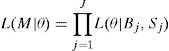
Under this model, the likelihood of observing B buys and S sells on a single trading day is:

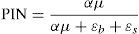
where B and S represent total buy trades and sell trades for the day, respectively, and θ = (α, δ, μ, ¿_b, ¿_s) is the parameter vector. This likelihood function is a mixture of three Poisson probabilities, weighted by the probability of having a “good news day” α(1 − δ), a “bad news day” αδ, and “no-news day” (1 − α). Assuming cross-trading day independence, the likelihood function across J days is just the product of the daily likelihood functions:

where B_j, and S_j are the numbers of buy and sell trades for day j = 1, …, J, and M = [(B₁, S₁), …, (B_J, S_J)] is the data set. Maximization of (2) over θ given the data M yields maximum likelihood estimates for the underlying structural parameters of the model (α, δ, μ, ¿_b, ¿_s). Once the parameters of interest are estimated, the Probability of Informed Trading, PIN, is calculated as:

where αμ + ¿_b + ¿_s is the arrival rate of all orders, αμ is the arrival rate of informed orders. The PIN is thus the ratio of orders from informed traders to the total number of orders.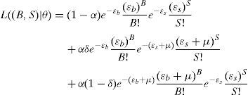

An attractive feature of the EKOP methodology is its apparently modest data requirement. All that is necessary to estimate the model is the number of buy- and sell-initiated trades for each stock and each trading day. However a shortcoming of the EKOP methodology is that, although the estimation procedure is straightforward, it often encounters numerical problems when performing the estimation in practice. Especially in stocks with a huge number of trades, the optimization program may bump into computational overflow or underflow (floating-point exception) and as a consequence it may not be able to obtain an optimal solution. Several numerical methods have been used for solving the maximization problem; for instance, Easley et al. (2010) and Lin and Ke (2011) propose two different factorizations of the likelihood function to facilitate numerical maximization. However, the convergence of optimization algorithm is not always possible and the method fails to deliver the PIN to certain active stocks. These difficulties in estimating PIN have worsened in the last year due to the steady increase in the number of trades which are a consequence, among other reasons, of the growth in automated trading and structural changes in the market that have greatly reduced market depth (Aslan et al., 2011).

3

VPIN model (Easley et al., 2012a)

The fundamental link between PIN and VPIN can be found in Easley et al. (2008). Departing from EKOP (1996) PIN model as a benchmark, these authors develop a dynamic econometric model of trading by introducing time-varying (GARCH-style) arrival rates of informed and uninformed traders. They show that for a particular period of time τ (e.g., days), the expected trade imbalance E[VτSell−VτBuy] approximates αμ (PIN numerator) while the expected total number of trades E[VτSell+VτBuy] equals αμ+εb+εs (PIN denominator).

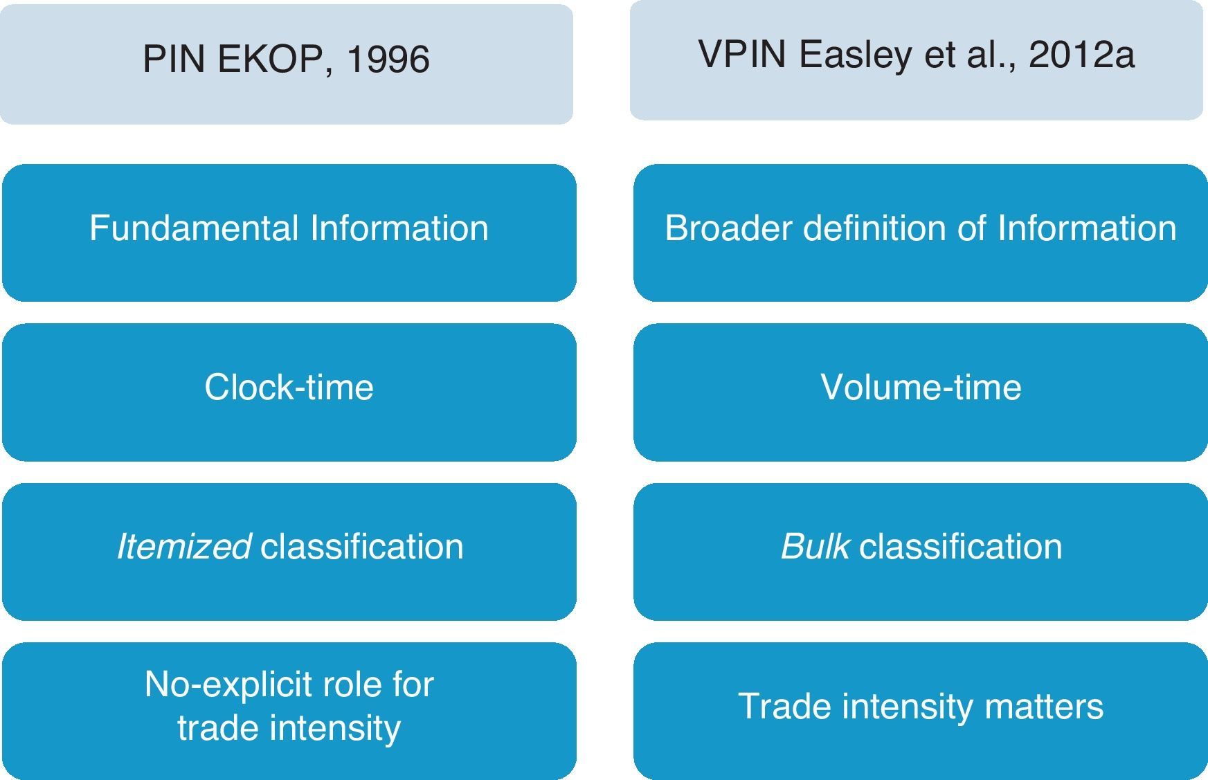
Before detailing the VPIN approach, Fig. 1 outlines the main innovations that Easley et al. (2012a) introduce regarding the original PIN model.

Fig. 1.

VPIN innovations. Figure outlines the four main innovations that Easley et al. (2012a) introduce in the VPIN model dealing with the PIN original model developed by EKOP (1996).

The first two innovations basically make reference to the update of the model to the high frequency environment. The first one is the broader definition of information that underlies VPIN. The PIN model focuses on fundamental information about the true value of the stock. In the PIN model, information about stock value arrives with a certain probability on a particular day. Then, informed traders emerge on the right side of the market unbalancing trading activity. VPIN measures order flow toxicity and toxicity is a wider concept focusing on the likelihood of HF liquidity providers being adversely selected. Adverse selection may include fundamental information but also other factors related to the nature of the trading in the overall market or to the specifics of liquidity demand over a particular interval. Therefore, information in VPIN is related to underlying events that provoke unbalanced or accelerated trade over a relatively short horizon including not only those related to asset returns, but also others reflecting more systemic or portfolio-based effects.

The second divergence is the different time system on which both models work. The PIN model works on clock-time while VPIN works on volume-time. The PIN model collects daily order imbalances under the assumptions of daily independence and price efficiency at the end of the day. In contrast, VPIN computes order imbalance on every occasion the market exchanges a constant amount of volume (volume bucket) mimicking the arrival to the market of news of comparable relevance. Sampling by volume is equivalent to dividing the trading session into periods of comparable information content reducing, in this way, the impact of volatility clustering in the sample.⁶

The third innovation supposes an “incidental contribution” (Easley et al., 2012a, p. 1459) that is beyond even the VPIN computation. In particular, the PIN model employs an itemized classification to distinguish between buy and sell volume while VPIN proposes a new approach labeled bulk classification. In the PIN model order imbalance is observed by signing tick-by-tick trades. The Lee–Ready algorithm is commonly used for this task in those markets where it is not possible to distinguish the aggressor's side of the trade. In VPIN, Easley et al. (2012a) argue that, particularly in high frequency settings, itemized approaches are problematic even if classification algorithms are not necessary at all. These authors propose to compute order imbalances by aggregating trades over short time intervals (time bars) or volume intervals (volume bars) and then using normal distribution and standardized price changes to determine the percentage of buy and sell volume. Nevertheless, VPIN computation is also possible using an itemized approach for raw data.⁷

Finally, in the original PIN model, order imbalances are observed in terms of number of buys and sells, regardless of the trade size.⁸ In contrast, VPIN takes into account trade size by treating each reported trade as if it were an aggregation of trades of unit size. This convention explicitly puts trade intensity into the analysis.

It is also important to mention that the output and estimation procedure of the models also differ. The PIN model provides a single estimation of the probability of informed trading for a particular period of time (year, month) that is obtained once non-observable parameters are estimated by maximum likelihood. VPIN procedure produces a serial of estimations of the VPIN metric for a time period and does not require intermediate estimation of non-observable parameters or the application of numerical methods. This serial measure also allows the capture of risk variations at intraday levels but taking into account that an individual VPIN observation is not relevant itself but only in reference to their empirical distribution. In this paper our main goal is to analyze PIN and VPIN compatibility so we focus more on aggregate VPIN metrics (average, median, standard deviation) than on particular values of this measure.

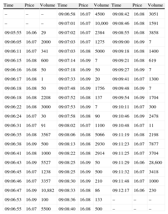
3.1

VPIN metric procedure

To illustrate VPIN estimation procedure we opt for using an example rather than repeat the specific formulation and the algorithm that are available in Easley et al. (2012a). We depart from a tick-to-tick sample of transactions of a particular instrument with the following information: time of the trade, price and volume exchanged. Table 1 shows a small excerpt of transaction data for one high frequently traded stock of the Spanish market, Telefónica (ticker “TEF”), on date 02/01/2009.

Table 1.

VPIN metric procedure – sample excerpt.

Time	Price	Volume	Time	Price	Volume	Time	Price	Volume
–	–	–	09:06:58	16.07	4500	09:08:42	16.08	3051
–	–	–	09:07:01	16.07	10,000	09:08:46	16.08	1591
09:05:55	16.06	29	09:07:02	16.07	2384	09:08:55	16.08	3858
09:06:05	16.07	2000	09:07:03	16.07	1275	09:09:00	16.09	7
09:06:11	16.07	341	09:07:03	16.08	5000	09:09:18	16.08	1400
09:06:15	16.08	600	09:07:14	16.09	7	09:09:21	16.08	619
09:06:16	16.08	50	09:07:18	16.09	50	09:09:27	16.09	7
09:06:17	16.08	1	09:07:33	16.09	20	09:09:41	16.07	1300
09:06:18	16.08	50	09:07:48	16.09	1756	09:09:48	16.09	7
09:06:18	16.08	2208	09:07:52	16.08	137	09:09:54	16.09	1704
09:06:22	16.08	3000	09:07:53	16.09	7	09:10:11	16.07	300
09:06:24	16.07	30	09:07:58	16.08	90	09:10:46	16.09	2478
09:06:31	16.07	91	09:08:02	16.07	1100	09:10:48	16.07	11
09:06:35	16.08	3567	09:08:06	16.08	5066	09:11:19	16.08	2198
09:06:38	16.09	500	09:08:13	16.08	2930	09:11:23	16.07	7877
09:06:41	16.08	1000	09:08:22	16.08	2914	09:11:25	16.07	3704
09:06:43	16.09	5527	09:08:25	16.09	50	09:11:29	16.06	28,600
09:06:45	16.07	1238	09:08:25	16.09	500	09:11:32	16.07	3418
09:06:46	16.07	3357	09:08:30	16.09	210	09:11:48	16.07	1000
09:06:47	16.09	10,882	09:08:33	16.08	86	09:12:17	16.06	230
09:06:53	16.09	100	09:08:36	16.08	133	–	–	–
09:06:55	16.07	5500	09:08:40	16.08	500	–	–	–

Table presents a small excerpt of the transaction data (time, price and volume) necessary to calculate VPIN. The data corresponds to several minutes on the first trading day of the year 2009 for a high frequently traded stock in the Spanish market (Telefónica, TEF).

3.1.1

Time (or volume) bars

The original procedure begins with trade aggregation in time (or volume) bars. Although this first step is not enforced and it is possible to work with raw transaction data, Easley et al. (2012a) assert that data aggregation leads to a better identification of buy and sell volume and thus, better flow toxicity estimates. Bar size is the first key variable of the VPIN computation process. Following Easley et al. (2012a) we use a 1-min time bar. In each time bar, trades are aggregated by adding the volume of all the trades in the bar (if any) and by computing price change for this period of time.⁹ After that and in order to take into account trade size, the sample is “expanded” by repeating each bar price change as many times as the volume in the bar. Thus, the original raw sample became a sample of one-unit trades each of them associated with the price change of the corresponding bar.

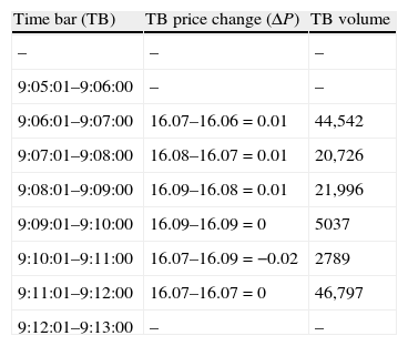
Table 2 shows Time Bar (TB) computation in our example. We can calculate six 1-min bars (from 9:07 to 9:12) from the small sample excerpt in our example. TB Volume is the accumulated volume of all transactions that take place in the corresponding minute and TB Price Change (ΔP) represents the variation of transaction price from the last price in the corresponding time bar to the last available in the previous one. The sample is then “expanded” by considering trades of one unit that are associated with the corresponding price change. For example, in time bar 9:07 instead of considering that we have a unique transaction of 44,542 shares we consider 44,542 (independent) one-unit trades, each of them associated with a price change of 0.01.

Table 2.

VPIN metric procedure – time bars.

Time bar (TB)	TB price change (ΔP)	TB volume
–	–	–
9:05:01–9:06:00	–	–
9:06:01–9:07:00	16.07–16.06 = 0.01	44,542
9:07:01–9:08:00	16.08–16.07 = 0.01	20,726
9:08:01–9:09:00	16.09–16.08 = 0.01	21,996
9:09:01–9:10:00	16.09–16.09 = 0	5037
9:10:01–9:11:00	16.07–16.09 = −0.02	2789
9:11:01–9:12:00	16.07–16.07 = 0	46,797
9:12:01–9:13:00	–	–

Table shows time bar completion in our example. Time Bar (TB) presents the 1-min time bars that can be computed from the example excerpt. TB Price Change (ΔP) reflects the price change that takes place in each bar. Finally, TB Volume is the aggregated volume of all trades that take place into the minute. This volume has the interpretation of the number of one-unit independent trades.

3.1.2

Volume buckets and bulk classification

Volume bucket (or volume bin) is the second essential variable in VPIN metric. Volume buckets represent pieces of homogeneous information content that are used to compute order imbalances. In Easley et al. (2012a) volume bucket size (VBS) is calculated by dividing the average daily volume (in shares) by 50 which is the number of buckets they initially consider. Therefore, if we depart from the average daily volume, it is the number of buckets which fully determines VBS. Consequently, we consider the number of buckets as our second key variable.

Buckets are filled by adding the volume in consecutive time bars until completing the VBS. If the volume of the last time bar needed to complete a bucket is for a size greater than required, the excess size is given to the next bucket. In general, a volume bucket needs a certain number of time bars to be completed although it is also possible that the volume in a time bar could be enough to fill one (or more) volume buckets.

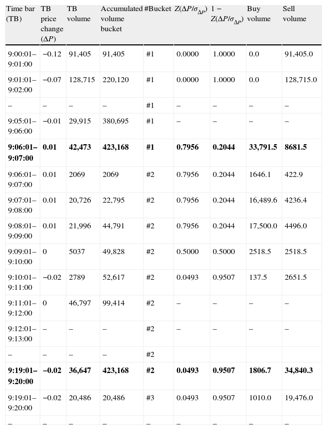
Table 3 shows the bucket assignation process. The average daily volume for TEF in 2009 was 21,158,426 shares. Following Easley et al. (2012a) we use 50 buckets and obtain a VBS of 423,168 shares. Bucket #1 starts to fill from the first time bar. When the volume of the 9:06 time bar is included, bucket #1 accounts for 380,695 shares and 42,423 shares are pending to complete it. The following time bar is 9:07 with an associated volume of 44,542 shares, 42,423 of which are used to complete bucket #1 and the remaining 2069 shares are assigned to the following bucket (bucket #2). Bucket #2 is completed in the 9:20 time bar.

Table 3.

VPIN metric procedure – volume bucketing and bulk classification.

Time bar (TB)	TB price change (ΔP)	TB volume	Accumulated volume bucket	#Bucket	Z(ΔP/σΔP)	1 − Z(ΔP/σΔP)	Buy volume	Sell volume
9:00:01–9:01:00	−0.12	91,405	91,405	#1	0.0000	1.0000	0.0	91,405.0
9:01:01–9:02:00	−0.07	128,715	220,120	#1	0.0000	1.0000	0.0	128,715.0
–	–	–	–	#1	–	–	–	–
9:05:01–9:06:00	−0.01	29,915	380,695	#1	–	–	–	–
9:06:01–9:07:00	0.01	42,473	423,168	#1	0.7956	0.2044	33,791.5	8681.5
9:06:01–9:07:00	0.01	2069	2069	#2	0.7956	0.2044	1646.1	422.9
9:07:01–9:08:00	0.01	20,726	22,795	#2	0.7956	0.2044	16,489.6	4236.4
9:08:01–9:09:00	0.01	21,996	44,791	#2	0.7956	0.2044	17,500.0	4496.0
9:09:01–9:10:00	0	5037	49,828	#2	0.5000	0.5000	2518.5	2518.5
9:10:01–9:11:00	−0.02	2789	52,617	#2	0.0493	0.9507	137.5	2651.5
9:11:01–9:12:00	0	46,797	99,414	#2	–	–	–	–
9:12:01–9:13:00	–	–	–	#2	–	–	–	–
–	–	–	–	#2
9:19:01–9:20:00	−0.02	36,647	423,168	#2	0.0493	0.9507	1806.7	34,840.3
9:19:01–9:20:00	−0.02	20,486	20,486	#3	0.0493	0.9507	1010.0	19,476.0
–	–	–	–	–	–	–	–	–

Columns 1–5 describe the bucket assignation process. Buckets are filled by adding the volume in consecutive time bars until reaching 423,168 shares which is the volume bucket size (VBS). If the volume of the last time bar needed to complete a bucket is for a size greater than required, the excess size is given to the next bucket. Bold rows indicate the time bar when a bucket is completed. Columns 6–9 display the probabilistic method to classify buyer- and seller-initiated volume for each time bar. Columns 6 and 7 present the value of normal distribution evaluated in the standardized price change (ΔP/σ_ΔP) and the complementary, respectively. Columns 8 and 9 are the result of multiplying TB Volume (column 4) by the value in columns 6 and 7, respectively.

At the same time of bucket completion, time bar volume is classified as buyer- or seller-initiated in probabilistic terms. Normal distribution is employed labeling as “buy” the volume that results from multiplying the volume bar by the value of the normal distribution evaluated in the standardized price change Z(ΔP/σ_ΔP). To standardize, we divide the corresponding price change by the standard deviation of all price changes for the whole sample. Analogously, we categorize as “sell” the volume that results from multiplying the volume bar by the complementary of the normal distribution for the buy side, 1 − Z(ΔP/σ_ΔP).

In the last columns of Table 3, we observe buy and sell distribution of volume bars in our example. The standard deviation of all price changes for our sample is 0.01211. For time bars with a null price change, the probabilistic method allocates one half of the volume as buy and one half as sell. The volume of the time bars with positive price changes are mainly classified as buy while the volume of the time bars with negative price changes are mainly classified as sell. The higher the price change in absolute terms the higher the asymmetry of the classified volume.

3.1.3

Order imbalance

Order imbalance (OI) is computed for each bucket by simply obtaining the absolute value of the difference between buy volume and sell volume in the assigned time bars.¹⁰

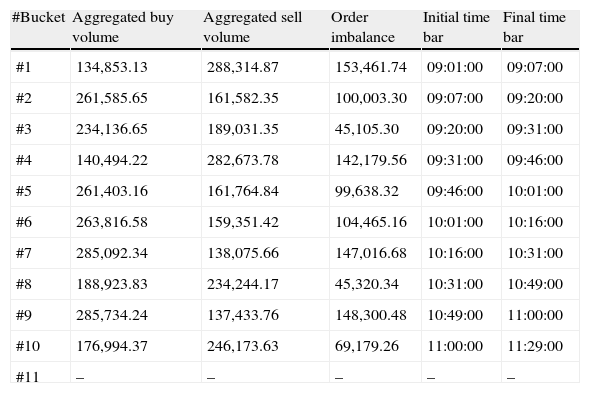
Table 4 shows order imbalance for the first ten buckets. It is important to point out that some buckets need short clock-time to be completed (e.g., bucket #1) while others need longer periods of time (e.g., bucket #10).

Table 4.

VPIN metric procedure – order imbalance.

#Bucket	Aggregated buy volume	Aggregated sell volume	Order imbalance	Initial time bar	Final time bar
#1	134,853.13	288,314.87	153,461.74	09:01:00	09:07:00
#2	261,585.65	161,582.35	100,003.30	09:07:00	09:20:00
#3	234,136.65	189,031.35	45,105.30	09:20:00	09:31:00
#4	140,494.22	282,673.78	142,179.56	09:31:00	09:46:00
#5	261,403.16	161,764.84	99,638.32	09:46:00	10:01:00
#6	263,816.58	159,351.42	104,465.16	10:01:00	10:16:00
#7	285,092.34	138,075.66	147,016.68	10:16:00	10:31:00
#8	188,923.83	234,244.17	45,320.34	10:31:00	10:49:00
#9	285,734.24	137,433.76	148,300.48	10:49:00	11:00:00
#10	176,994.37	246,173.63	69,179.26	11:00:00	11:29:00
#11	–	–	–	–	–

Table presents order imbalances for the first ten buckets for TEF in the year 2009. Aggregated Buy (Sell) Volume is the sum of all buy-initiated (sell-initiated) volume of the corresponding time bars for each bucket. The sum of both columns in each row equals the VBS. Order Imbalance is the difference between values in columns 2 and 3. Finally, the lasts two columns indicate the initial and the final time bar of the corresponding bucket, respectively.

3.1.4

VPIN and sample length

In the last step we finally obtain VPIN values. To do that, it is necessary to define a new variable: sample length (n). This variable establishes the number of the buckets with which VPIN is computed. Following the link established in Easley et al. (2008).

where VPIN is simply the average of order imbalances in the sample length, that is, the result of dividing the sum of order imbalances for all the buckets in the sample length (proxy of the expected trade imbalance) by the product of volume bucket size (VBS) multiplied by the sample length (n) (proxy for the expected total number of trades). VPIN metric is updated after each volume bucket in a rolling-window process. For example, if the sample length is 50, when bucket #51 is filled, we drop bucket #1 and we calculate the new VPIN based on buckets #2 to #51. Easley et al. (2012a) firstly consider sample length equal to the number of buckets (50), but throughout the paper the authors change this variable to 350 or 250 depending on what they want to analyze. A sample length of 50 buckets when the number of buckets is also 50 is equivalent to obtaining a daily VPIN. A sample length of 250 (350) when the number of buckets is 50 is equivalent to obtaining a five-day (seven-day) VPIN.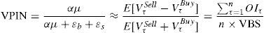

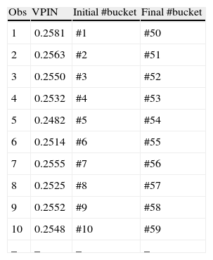
Table 5 shows the first ten VPIN values for TEF in the year 2009 using a sample length of 50 buckets (n = 50). As 50 buckets are necessary to obtain VPIN, our first value of VPIN is obtained once bucket #50 is filled.

Table 5.

VPIN metric procedure – VPIN and sample length.

Obs	VPIN	Initial #bucket	Final #bucket
1	0.2581	#1	#50
2	0.2563	#2	#51
3	0.2550	#3	#52
4	0.2532	#4	#53
5	0.2482	#5	#54
6	0.2514	#6	#55
7	0.2555	#7	#56
8	0.2525	#8	#57
9	0.2552	#9	#58
10	0.2548	#10	#59
–	–	–	–

Table presents the first ten values of VPIN for TEF in the year 2009. VPIN is computed using 1-min time bars, 50 volume buckets and a sample length (n) of 50 buckets. VPIN is the ratio between the expected trade imbalance (approximated by the sum of the bucket order imbalances in the sample length) and the expected total number of trades (approximated by volume bucket size, VBS, multiplied by the sample length), VPIN=αμαμ+εb+εs≈E[VτSell−VτBuy]E[VτSell+VτBuy]=∑τ=1nOIτn×VBS

VPIN metric is updated after each bucket completion in a rolling-window process. Thus, when bucket 51 is filled, we drop bucket #1 and calculate a new VPIN observation focus on buckets #2 to #51.

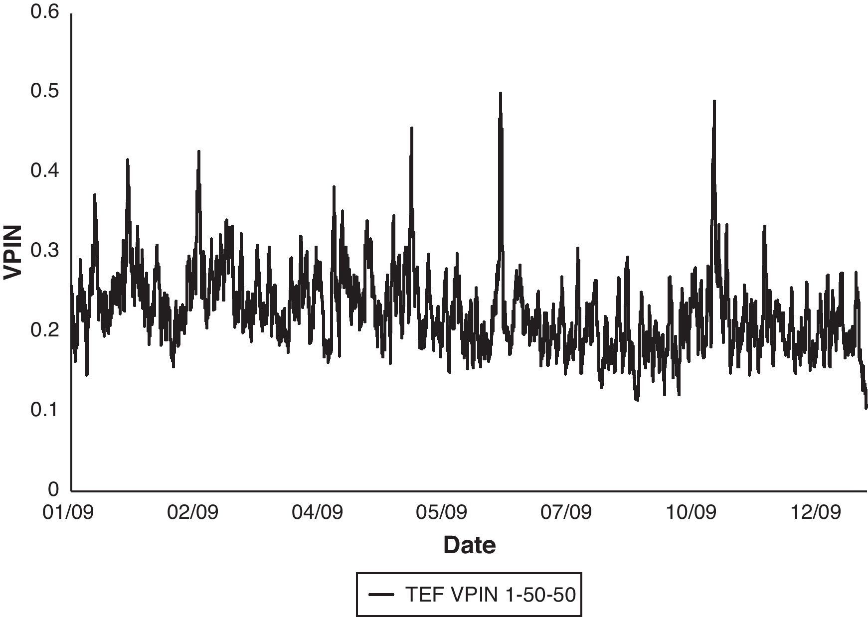
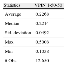
Finally, Fig. 2 shows the complete VPIN series for TEF in the year 2009 using 1-min time bars, 50 buckets to compute the VBS and 50 buckets as sample length. Table 6 reports basic statistics of this series.

Fig. 2.

Telefónica (TEF) VPIN 2009. Figure shows VPIN series for TEF in the year 2009 using 1-min time bars, 50 buckets to compute the VBS and 50 buckets as sample length (TEF VPIN 1-50-50).

Table 6.

TEF VPIN 2009 statistics.

Statistics	VPIN 1-50-50
Average	0.2268
Median	0.2214
Std. deviation	0.0492
Max	0.5008
Min	0.1038
# Obs.	12,650

Table reports basic statistics for VPIN series of TEF stock in the year 2009 using 1-min time bars, 50 buckets to compute the VBS and 50 buckets as sample length (TEF VPIN 1-50-50).

To summarize the VPIN estimation procedure, we briefly review the three levels in which the VPIN calculation takes place: (1) buy and sell classification occurs at bar level (time or volume) where bar size is the key variable. At this level, individual trades are aggregated and the resulting volume is then classified as buyer- or seller-initiated using a probabilistic method based on normal distribution and standardized price change. This level is what Easley et al. (2012a) denominate Bulk classification. Regarding bar size, the authors show that within reasonable bounds the choice of the amount of time contained in a time bar has little effect in measuring order imbalances. (2) Order imbalance is computed in absolute terms at bucket level where the number of buckets is the key variable. Working in volume-time provides a more accurate scenario with which to accomplish HFT strategies (Easley et al., 2012b) with volume buckets representing units of homogeneous information. In our opinion, this is the more relevant variable of VPIN metric procedure. In principle, there is no formal justification in Easley et al. (2012a) for choosing 50 buckets or any other specific quantity. It seems clear that when the number of buckets is high enough, resulting order imbalances may be capturing the different components of the adverse selection risk faced by HF liquidity providers. However, it seems unclear what kind of toxicity is measured when a lower number of buckets is employed. For example, if we opt to work with one bucket, by definition, we are computing a daily order imbalance on average which is quite similar to the PIN model where order imbalances are computed on a daily basis. Therefore, it is possible that the information content (and thus, the nature of toxicity) differs from a VPIN computed using one bucket to another VPIN computed using a higher number of buckets. (3) Finally, VPIN values are approximated by the average of a particular number of bucket order imbalances in a rolling-window process. Sample length is the key variable in this level and, once again, there is no formal discussion for using a particular value for this variable.

4

Market description, data, and sample

Our sample is made up of stocks traded on the electronic trading platform of the Spanish Stock Exchange, known as the SIBE (Sistema de Interconexión Bursátil Español). The SIBE is an order-driven market where liquidity is provided by an open limit order book. Trading is continuous from 9:00 am to 5:30 pm. There are two regular call auctions each day: the first one determines the opening price (8:30-9:00 am), whereas the second one sets the official closing price (5:30-5:35 pm). A continuous session could be interrupted by a system of stock-specific intraday price limits and short-lived call auctions directed to handle unusual volatility levels. In all auctions (open, close and volatility) orders can be submitted, modified or canceled, but no trades occur. Three basic types of orders are allowed: limit orders, market orders, and market-to-limit orders. In the continuous session, a trade occurs whenever an incoming order matches one or more orders on the opposite side of the limit order book. Orders submitted that are not instantaneously executed are stored in the book waiting for a counterparty according to a price-time priority rule. Unexecuted orders can always be canceled and modified.

Trade and quote data for this study come from SM data files provided by Sociedad de Bolsas, S.A. SM files comprise detailed time-stamped information about the first level of the limit order book for each stock listed on the SIBE. Any trade, order submission or cancelation that affects best prices in the book generates a new record. The distinction between buyer-initiated and seller-initiated trades is straightforward, without the need to use any classification algorithm.

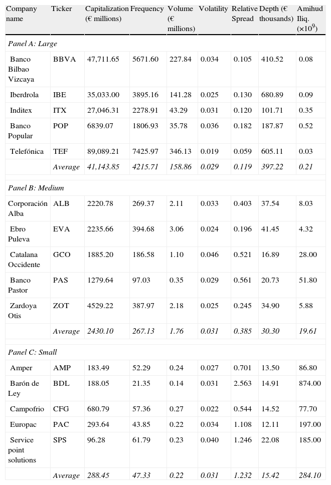
Our sample comprises 15 Spanish stocks for the year 2009 split into three 5-stock portfolios typifying different levels of capitalization, activity and liquidity (large, medium and small). To do that, the five stocks of each portfolio were chosen at random from those belonging the entire year to the IBEX-35 index, the IBEX MEDIUM CAP index, and the IBEX SMALL CAP index, respectively. The IBEX-35 index comprises the biggest, most liquid and frequently traded stocks in the SIBE, whereas the stocks in the other two indexes are smaller, less frequently traded and more illiquid.¹¹

In Table 7, we provide sample statistics on several commonly-used market indicators of trading activity, volatility and liquidity. As expected, market capitalization, trading activity and liquidity decreases as we move from the large portfolio to the small one. Overall, we observe that stocks in the large portfolio are on an average much more traded and liquid than the stocks belonged to the other two groups. In any case, we test the equality of the different market indicators between the three portfolios (Kruskal-Wallis test) and between each pair (Mann-Whitney test). All the tests performed are rejected at 5% significance level with the exception of those related with the volatility proxy (not reported but available upon request).

Table 7.

Sample statistics.

Company name	Ticker	Capitalization (€ millions)	Frequency	Volume (€ millions)	Volatility	Relative Spread	Depth (€ thousands)	Amihud Iliq. (×10^9)
Panel A: Large
Banco Bilbao Vizcaya	BBVA	47,711.65	5671.60	227.84	0.034	0.105	410.52	0.08
Iberdrola	IBE	35,033.00	3895.16	141.28	0.025	0.130	680.89	0.09
Inditex	ITX	27,046.31	2278.91	43.29	0.031	0.120	101.71	0.35
Banco Popular	POP	6839.07	1806.93	35.78	0.036	0.182	187.87	0.52
Telefónica	TEF	89,089.21	7425.97	346.13	0.019	0.059	605.11	0.03
	Average	41,143.85	4215.71	158.86	0.029	0.119	397.22	0.21
Panel B: Medium
Corporación Alba	ALB	2220.78	269.37	2.11	0.033	0.403	37.54	8.03
Ebro Puleva	EVA	2235.66	394.68	3.06	0.024	0.196	41.45	4.32
Catalana Occidente	GCO	1885.20	186.58	1.10	0.046	0.521	16.89	28.00
Banco Pastor	PAS	1279.64	97.03	0.35	0.029	0.561	20.73	51.80
Zardoya Otis	ZOT	4529.22	387.97	2.18	0.025	0.245	34.90	5.88
	Average	2430.10	267.13	1.76	0.031	0.385	30.30	19.61
Panel C: Small
Amper	AMP	183.49	52.29	0.24	0.027	0.701	13.50	86.80
Barón de Ley	BDL	188.05	21.35	0.14	0.031	2.563	14.91	874.00
Campofrio	CFG	680.79	57.36	0.27	0.022	0.544	14.52	77.70
Europac	PAC	293.64	43.85	0.22	0.034	1.108	12.11	197.00
Service point solutions	SPS	96.28	61.79	0.23	0.040	1.246	22.08	185.00
	Average	288.45	47.33	0.22	0.031	1.232	15.42	284.10

Table presents the 15 stocks included in the sample grouped in three 5-stock portfolios: Large (stocks from IBEX35 index in Panel A), Medium (stocks from IBEX MEDIUM CAP index in Panel B), and Small (stocks from IBEX SMALL CAP index in Panel C). For each stock, the table reports the market capitalization at the end of 2009 and the mean of different daily indicators of trading activity, volatility, and liquidity. Activity proxies are the number of trades (frequency) and the traded volume in millions of Euros. Volatility proxy is the high-low quote midpoint ratio. Liquidity measures are the relative spread and market depth (bid + ask) in thousands of Euros. Both liquidity measures are daily mean weighted by time. Amihud Iliq. is the measure of illiquidity proposed by Amihud (2002) which consists of the mean of the daily ratio between return and traded volume.

5

Empirical evidence: PIN and VPIN comparison

In this section we compare the VPIN model with its predecessor PIN by applying both methods to the same stock sample. As we have discussed, both models are based on the observation of order imbalances to measure the probability of being adversely selected. VPIN is introduced as the updated version of PIN in a double sense: (1) as a new tool designed to deal with the new risks from the new market paradigm of HFT, and (2) as a straightforward approach to obtain the probability of being adversely selected while avoiding the most important drawbacks of the PIN model. In the previous section, we have reviewed VPIN procedure paying special attention to the main innovations introduced and the key variables for its computation. By comparing PIN and VPIN in this section our main goal is to stress the role of VPIN as an easy way to measure adverse selection (or order flow toxicity) not only to the HFT environment.

We estimate first the PIN model via maximum likelihood for each stock and month in 2009. Easley et al. (1997a) indicate that a 30 trading-day window allows sufficient trade observations for the PIN estimation procedure. Akay et al. (2012) use 20 trading days to estimate PIN finding numerical solutions for all their estimations. Hence, the use of one-month transaction data (around 20 trading days) should be wide enough to produce reliable estimates. We use the optimization algorithm of the Matlab software to maximize the likelihood function in (2). We usually run the maximum likelihood function 100 times for each stock-month pair in our sample, except for several months of large stocks for which we increase the iterations to 1000 to ensure that a maximum is reached. We follow Yan and Zhang (2012) to set initial values for the five parameters in the likelihood function. The estimation procedure converges for virtually all the 60 stock-month combinations of our sample.

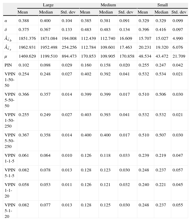
Summary statistics for PIN parameters and PIN values are reported in Table 8. First, we compute mean values across months for each stock and then, we report the cross-sectional mean, median and standard deviation for each portfolio. As expected, we find that the probability of informed trading increases as we move to lower levels of trading activity and liquidity. The mean (median) results show that PIN is 0.102 (0.098) for large portfolio, rising to 0.160 (0.158) for medium, and it reaches 0.255 (0.247) for the stocks included in the small portfolio. These results are consistent with EKOP (1996) findings, and also with those of Abad and Rubia (2005) who also analyze the PIN model for the Spanish stock market. The analysis of PIN parameters can provide more information about the origin of the observed differences in PIN values among portfolios. According to Eq. (3), PIN is positively related to the probability of an information event (α) and negatively related to the ratio of the arrival rate of uninformed trades to the arrival rate of informed trades ((¿_b + ¿_s)/μ). From Table 8 we can observe similar α value in the three portfolios. Using Kruskal–Wallis and Mann-Whitney tests (not reported) we reject that this probability statistically differs among the three groups. On the contrary, we can observe how the uninformed-to-informed ratio dramatically decreases as we move from the most active to the less frequently traded stocks (using mean values, from 2.60 for large stocks to 1.32 for medium, being 0.74 for small stocks). Hence, our results suggest that asymmetric information risk is higher for the more illiquid and less frequently traded stocks due to the fact that proportionally there are fewer uninformed traders, which increases the probability of trading with an informed trader (consistent with Abad and Rubia, 2005).¹²

Table 8.

PIN and VPIN statistics.

	Large			Medium			Small
	Mean	Median	Std. dev	Mean	Median	Std. dev	Mean	Median	Std. dev
α	0.388	0.400	0.104	0.385	0.381	0.091	0.329	0.329	0.099
δ	0.375	0.367	0.133	0.483	0.483	0.134	0.396	0.416	0.097
¿b	1851.376	1871.084	194.008	112.439	112.740	16.609	15.707	15.027	4.990
¿s	1962.931	1952.498	254.256	112.784	109.601	17.463	20.231	19.320	6.076
μ	1469.629	1199.510	894.473	170.853	109.905	170.858	48.534	43.472	21.709
PIN	0.102	0.098	0.029	0.160	0.158	0.020	0.255	0.247	0.042
VPIN 1-50-50	0.254	0.248	0.027	0.402	0.392	0.041	0.532	0.534	0.021
VPIN 5-50-50	0.366	0.357	0.014	0.399	0.399	0.017	0.510	0.506	0.030
VPIN 1-50-250	0.255	0.249	0.027	0.403	0.393	0.041	0.532	0.532	0.021
VPIN 5-50-250	0.367	0.358	0.014	0.400	0.400	0.017	0.510	0.507	0.030
VPIN 1-1-5	0.061	0.064	0.010	0.126	0.118	0.033	0.239	0.219	0.047
VPIN 5-1-5	0.082	0.078	0.013	0.128	0.123	0.030	0.248	0.237	0.057
VPIN 1-1-20	0.058	0.053	0.011	0.126	0.121	0.032	0.240	0.221	0.045
VPIN 5-1-20	0.082	0.077	0.013	0.128	0.125	0.030	0.248	0.237	0.055

Table presents the cross-sectional statistics of the estimated parameters of the PIN model, PIN values and eight VPIN series using different specifications of the key variables. The parameter α represents the probability that an information event will occur on a particular day, δ is the probability that an information event will be negative, ¿_b and ¿_s are the arrival rates of uninformed buyers and sellers, respectively, and μ represents the arrival rate of informed traders on information days. PIN is the probability of informed trade. The three digits that appear beside the acronym VPIN make reference to time bar size (min), number of buckets and sample length, respectively.

Regarding VPIN, we work with eight different combinations of the key variables. In particular, two VPIN series are obtained following the original model in Easley et al. (2012a), that is, 50 buckets to compute VBS and 50 buckets as sample length. For the first one, we employ 1-min time bars while the second is computed using 5-min time bars. We denote them as VPIN 1-50-50 and VPIN 5-50-50, respectively. To analysis the effects of changes in sample length, we also compute the previous two VPIN series by using a sample length of 250 (VPIN 1-50-250 and VPIN 5-50-250). Four additional series are also calculated by changing the number of the buckets and the sample length. In particular, for series of 1-min and 5-min time bars we use 1 bucket to compute the VBS (proxy for a daily order imbalance), and for sample length we use alternatively 5 buckets (proxy for a weekly VPIN) and 20 buckets (proxy for a monthly VPIN). We denote them as VPIN 1-1-5, VPIN 5-1-5, VPIN 1-1-20, and VPIN 5-1-20, respectively. Our aim is twofold: first, we are interested in analyzing how VPIN metric differs as we use different values of the key variables. Second, we propose values for the key variables that seem to better accomplish the PIN model. As we have discussed, the use of 1 bucket to compute the volume bucket size corresponds to obtaining a daily order imbalance on average, similar to the frequency used for order imbalances in the PIN model.

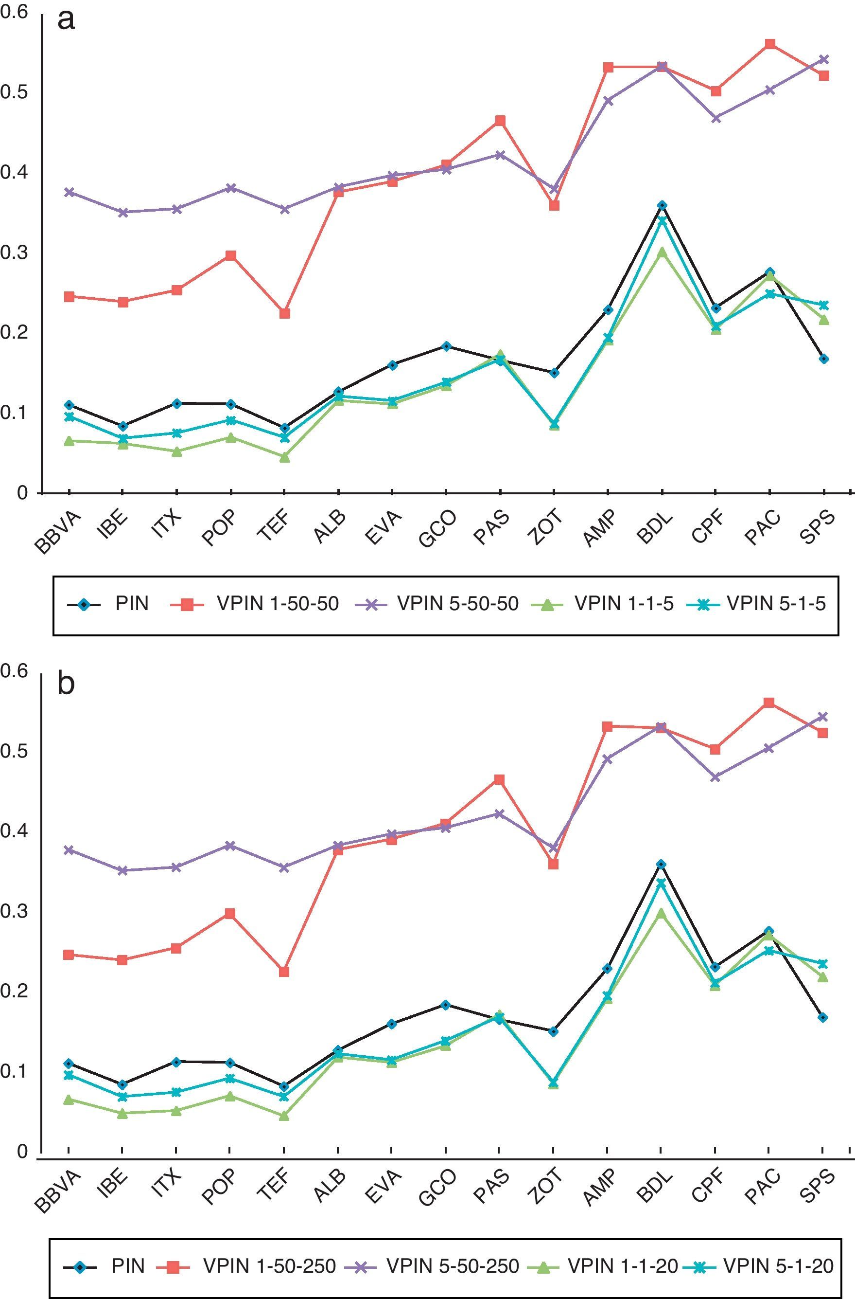
For each stock in our sample we compute mean values across the series for each VPIN specification. Table 8 reports the cross sectional mean, median and standard deviation for each portfolio. Firstly, similar to the PIN results, Table 8 shows VPIN values increasing from the more active stocks to infrequently traded ones; e.g., VPIN 1-50-50 mean (median) is 0.254 (0.248) for large stocks, it rises to 0.376 (0.392) for medium, and it reaches 0.532 (0.534) for small stocks. Secondly, when we compare the VPIN values obtained using different bar sizes, we observe higher values of VPIN with 5-min bars for the large portfolio. However, for the medium and small stock portfolios, VPIN calculated with 1-min and VPIN with 5-min bars present similar values. These results suggest that the variable bar size is more relevant for high frequently traded stocks. It is possible that 5 min might not be a reasonable size for active stocks with an elevated number of trades in short time intervals. On the contrary, for stocks with a lower number of trades during the day, working with longer bars seems to have little repercussion on VPIN values. Thirdly, we find that the influence of another two key variables, the number of buckets and sample length, on the estimate VPIN is quite different for each of them. We observe that increasing the size of sample length does not affect VPIN values. For instance, as seen in Table 8 the values of VPIN1-50-50 (VPIN1-1-5) are very similar to those of VPIN1-50-250 (VPIN1-1-20). However, we find significant differences in VPIN values when the number of buckets to calculate VBS changes. We observe a systematically higher VPIN for the original model of Easley et al. (2012a) with 50 buckets than when we calculate VPIN using this key variable mimicking EKOP (1996) PIN model with only 1 bucket. These results confirm our perception of VPIN measuring different toxicity (or adverse selection risk) depending on the value of number of buckets. Fig. 3 confirms this intuition. For the 15 stocks in our sample, Fig. 3a plots the PIN and four VPIN values (VPIN1-50-50, VPIN5-50-50, VPIN1-1-5, and VPIN5-1-5), while Fig. 3b plots the values of PIN and the same previous four specifications of VPIN but increasing the sample length. Fig. 3 shows that PIN and VPIN series estimated using 1 bucket for VBS, independently of the sample length, follow a similar pattern to the PIN values. Furthermore, cross-section correlation between PIN and VPIN values using 1 bucket to compute order imbalance is around 0.93.

Fig. 3.

PIN and VPIN. Figure plots the PIN and the eight VPIN values for the 15 stocks in our sample. The three digits that appear beside the acronym VPIN make reference to time bar size (min), number of buckets and sample length, respectively.

6

Concluding remarks

“HFT is here to stay” (Easley et al., 2012c, p. 27). Whereas several researchers focus on the unavoidable debate about the pros and cons of this growing activity worldwide, other researchers are embarking on the design of new tools to deal with the different demands arising from this new paradigm. Easley, López de Prado and O’Hara belong to this second group. Departing from the well-known PIN model to measure the probability of informed trading, these authors developed a new tool called Volume-Synchronized Probability of Informed Trading or VPIN to measure order flow toxicity in the market. Order flow toxicity is an old friend named adverse selection but in the context of the risks faced by a strategic HF liquidity provider. Thus, VPIN is introduced as the updated version of the PIN model incorporating a number of innovations primarily to deal with the HFT idiosyncrasy and, at the same time, offering a more tractable metric for adverse selection. In this paper, we look first at the PIN model to introduce by comparison the four main innovations of the VPIN metric: the broader definition of information, sampling in volume-time, bulk classification of buys and sells, and the incorporation of trade size. Then, using an example, we review the VPIN approach paying special attention to the three steps of this procedure: time bars, volume buckets and VPIN, and the corresponding key variables: bar size, number of buckets and sample length. By acquiring a better understanding of all this procedure, we recognize the usefulness of the VPIN method as a broad measure of adverse selection (or toxicity) which is not only circumscribed to the HFT environment. In other words, by setting the right values for the key variables – especially for the number of buckets – we are computing order imbalances that are capturing different information contents and hence, different risks of being adversely selected.

To illustrate this idea we estimate PIN and VPIN models for a sample of 15 Spanish stocks divided into three 5-stock size portfolios (large, medium and small). PIN values are obtained once the non-observable parameters of the model are estimated by maximum likelihood. Our PIN findings are consistent with those reported in EKOP (1996) and Abad and Rubia (2005) about higher probabilities of informed trading associated with less frequently traded stocks. For VPIN, we employ several specifications by varying the values of the keys variables. Our main results can be summarized as follows: (1) similar to the PIN model, higher VPIN values are observed for less frequently-traded stocks, (2) bar size choice seems to be only relevant for active stocks, (3) sample length have no repercussion in aggregated VPIN values, (4) the number of buckets to calculate the VBS greatly affects estimations of VPIN metric, and (5) the VPIN values obtained from the specification that emulates PIN model seem to successfully fit the original PIN estimations. Based on these results, we conclude that different specifications of the VPIN model could be used as different proxies for adverse selection with different information content. VPIN specifications employing lower VBS to compute order imbalance may incorporate transitory as well as permanent information, whereas VPIN specifications that consider higher VBS to compute order imbalance may mainly incorporate fundamental information about stocks (as in PIN model). These findings strengthen the value of the VPIN approach as a broad measure of adverse selection which is not exclusively applicable to the HFT world.