


Many firms choose to refinance their debt. We investigate the long run effects of this extended practice on credit ratings and credit spreads. We find that debt refinancing generates systematic rating downgrades unless a minimum firm value growth is observed. Deviations from this growth path imply asymmetric results. A lower firm value growth generates downgrades and a higher firm value growth generates upgrades, as expected. However, downgrades tend to be higher in absolute terms. We also find that the inverse relation between credit spreads and risk free rate that structural models usually predict still holds in this setting, but only in the short run. This negative relation will turn to be null in the medium run and positive in the long run.
Many different reasons may be behind the decision of a particular firm to issue new debt: financing a new investment project, getting funds to operate in a period of low earnings, or simply refinancing existing debt. The purpose of the issue is not irrelevant. An example is provided by Gande et al. (1997), who examine differences in debt securities underwritten by Section 20 subsidiaries of bank holding companies relative to those underwritten by investment houses. Among other results, they find that when debt is used to refinance existing debt, the credit spread is on average 14 basis points above the one that results considering “other purposes”. Intuitively, if the purpose of the issue is to finance a new investment project that will increase the expected earnings of the firm, and its market value, then the risk premium should be lower than in the case in which debt proceeds are used to refinance existing debt, because in this situation no added value is created.1 Refinancing current debt, however, seems to be one of the most important – if not the first – reason to issue new debt. The mentioned article for instance considers a sample in which 43.5% of the issues had the purpose to refinance existing debt. More evidence in this line is given by Hansen and Crutchley (1990), who investigate the relationship between corporate earnings and sales of common stocks, convertible bonds, and straight bonds. In this case, 64% of straight bond issues were used at least partially to refinance existing debt. This ratio grows up to 72% when they consider convertible debt.
In spite of the fact that debt refinancing appears as an extending practice, we know little about how this can potentially affect the credit standing of a firm in the long run. The present article represents a first attempt in this direction. We introduce the concept of refinancing contract, modeling dividend rates, maturities, and nominal debt payments, as part of this contract. We then describe the credit spreads faced by the firm to refinance as a function of the firm characteristics and the specific contract selected, and analyze how the fact that firms choose to refinance their debt can potentially affect the credit rating and the credit spreads of those firms in the long run.
The main conclusions of the paper are the following. First, debt refinancing generates systematic credit rating downgrades unless a minimum firm value growth is observed. Deviations from such a firm value growth path imply asymmetric results. While a lower firm value growth results in systematic downgrades and a higher firm value growth in systematic upgrades, as expected, the same deviation will have a higher effect in absolute terms when it is negative than when it is positive. Said in other words, we should expect rating migrations to exhibit a certain degree of inertia among those companies that choose to refinance their debt, and this inertia should be stronger in the case of downgrades than in the case of upgrades. Evidence in this regard has been actually provided by Altman and Kao (1992). Specifically, they find positive autocorrelation in S&P downgrades and upgrades for high-yield bonds, being this autocorrelation stronger in the case of downgrades.
The second main conclusion of the paper is that the traditional prediction of an inverse relation between credit spreads and risk free rate (Merton, 1974; Leland, 1994; Longstaff and Schwartz, 1995) holds just in the short run. Debt refinancing makes such relation to turn null in the medium run and positive in the long run. Evidence of this dynamic relation is in fact provided by Longstaff and Schwartz (1995) (negative effect in the short run) and Guha et al. (2001) (positive effect in the long run). Overall, we conclude that the common practice of debt refinancing and results provided in this paper allow explaining, in a unified framework, the empirical evidence on the dynamic relation between risk free rate and credit spreads.
The rest of the article is organized as follows: Section 2 introduces the concept of refinancing contract, and describes when, and how, a contract of this type with an arbitrary number of future payment dates n, can be designed. Section 3 analyzes the effects of debt refinancing under the specific cases of n=1 and n=2.2 Finally Section 4 summarizes the main findings of the paper.
2The general caseThe following assumption summarizes our theoretical framework.Assumption A A1: There are no taxes, problems concerning indivisibility, bankruptcy costs, transactions costs, or agency costs. A2: Trading takes place continuously. A3: There exists a risk free asset with constant interest rate r, that applies for borrowing and lending, and for any maturity. A4: Every individual acts as if she can buy or sell as much of any security as she wishes without affecting the market price. A5: Individuals may take short positions in any security, including the risk free asset, and receive the proceeds of the sale. Restitution is required for payouts made to securities held short. A6: Modigliani–Miller Theorem obtains, that is, the firm value is independent of its capital structure. A7: The firm value, V, follows the diffusion process given by
where μ is the expected rate of return on V, δ is the constant rate of firm value which is paid to equity holders as dividends, σ is the volatility of the rate of return which will be assumed to be constant, and z is a standard Brownian motion.

No assumption is made at this moment about the profile of nominal payments that constitute the corporate debt. We simply assume that a debt contract was signed at some period prior to current period t. Under this contract, at least a certain debt payment has to be satisfied at some future period τ>t. This, and any posterior debt payment, is to be financed by issuing additional equity. Under these conditions the equity and debt values will be a function of the firm value and time. Denote then the equity value as S(V,t), and the debt value as F(V,t). We start by defining the general form of any refinancing contract.Definition A refinancing contract between the firm and the debt holders at τ, is a vector Θ≡(δ,Ψ,ϒ)∈ℜ×ℜn×ℜn, with n<∞, by which: The firm, which is assumed to maximize equity holders’ wealth, promises (under limited liability) the payment of Ψ at ϒ, that is, the payment of ψi at τi, where ψi∈Ψ, τi∈ϒ, i=1, …, n, and τ1>τ. The firm also restricts itself to apply a dividend rate equal to δ, and loses the right to issue new debt. These restrictions apply until Θ has been canceled, either by satisfying nominal payments regularly (issuing new equity), or by means of a posterior debt refinancing contract. The debt holders renounce to F(V,τ).
We say that Θ is feasible, if and only if the firm and the debt holders are willing to sign Θ. The set of feasible Θ is denoted by ΘF.
A refinancing contract (RC) is therefore similar to a standard debt contract. The main difference is that debt holders do not provide cash to the firm at issuance, but the renounce to the payment of current debt (covenant c). In addition, we include an agreement on dividends (covenant b). This agreement prevents equity holders from extracting a higher share of the firm value (with the implied reduction for debt holders), by increasing the dividend rate after signing the contract.
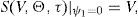
The following lemma establishes a necessary condition for a feasible set of refinancing contracts to exist.Lemma Let S(V,Θ,τ) and F(V,Θ,τ) denote the equity and debt value at τ when the value of the firm is V, the debt profile consists on the payment of Ψ at ϒ, and the dividend rate is δ. Then, Θ∈ΘFif and only if S(V,Θ,τ)=S(V,τ), implying S(V,τ)>0 as a necessary condition for a feasible Θ to exist. See Appendix A.
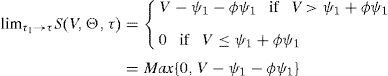
Although a formal statement of the proof is in the appendix, the intuition is straightforward. Modigliani and Miller's Theorem implies that no value is created or destroyed in the firm by refinancing its debt. As a consequence, equity holders can neither gain, nor lose due to refinancing. If they are worst off with the contract they will simply refuse it, but if they are better of this means that debt holders are worst off, and in this case they will be those who refuse the contract. This allows us to identify the set of feasible refinancing contracts with the set of contracts that leave equity holders with the same value. On the other hand, limited liability makes the equity value to be strictly positive if no current debt payment has to be satisfied, which is the case after signing the contract. This makes S(V,τ)>0 finally to be a necessary condition for a feasible contract to exist. One implication is that equity and debt can still be valued assuming that debt will be paid by issuing additional equity. The reason is that the possibility of refinancing will not alter their welfare with respect to this situation in any sense. We set up this argument as follows:Remark Refinancing does not alter neither equity holders, nor debt holders’ wealth. This implies that S(V,Θ,τ) and F(V,Θ,τ) can be valued assuming that debt payments are to be financed by issuing new equity, even if this never happens, that is, even if the firm always chooses to refinance its debt. Searching for a feasible contract implies at this point searching for 2n+1 elements. The following restriction on the relation between debt payments, and on the time spread between these payments, will allow us to reduce the dimension of the problem to 3. Let Ψ=ψ1Φ, where Φ is the n-dimensional vector which first element ϕ1 equals 1, and the remaining are some fixed values ϕi>0 ∀i≥2. Let also Π=(τ1−τ)Λ, where Π denotes the n-dimensional vector which first element π1 equals (τ1−τ), and πi equals (τi−τi−1) ∀i≥2. Λ on the other hand denotes the n-dimensional vector which first element η1 equals 1, and the remaining are some fixed values ηi>0 ∀i≥2. If we denote Δ≡(n,Φ,Λ) the vector that describes a particular corporate debt structure, then, for any Δ, (δ,Ψ,ϒ)∈ℜ×ℜn×ℜn is in fact fully described by (δ,ψ1,τ1)∈ℜ×ℜ×ℜ. The following assumption describes the behavior of the equity value as a function of these three elements. Although this behavior is stated as an assumption, it will be shown to hold later on for the specific cases of n=1 and n=2. B1:S(V,Θ,τ) is a continuous and strictly decreasing function in ψ1 (CSD (ψ1)), with S(V,Θ,τ)|ψ1=0=V, and limψ1→∞S(V,Θ,τ)=ER.N.∫ττ1δV(s)e−r(s−τ)ds=V(1−e−δT1).3 B2:S(V,Θ,τ) is a continuous and strictly increasing function in τ1 (CSI (τ1)), with limτ1→τS(V,Θ,τ)=Max0,V−∑i=1nψi,4 and limτ1→∞S(V,Θ,τ)=V. Denote ψˆ1 the ψ1 value such that S(V,τ)=V−ψ1∑i=1nϕi, that is, ψˆ1=F(V,τ)/∑i=1nϕi. B3:S(V,Θ,τ) is a continuous and strictly increasing function in δ (CSI (δ)), with limδ→∞S(V,Θ,τ)=V.
Assumption B1 asserts that the equity value is a continuous and strictly decreasing function in the nominal payments that equity holders have to satisfy. S(V,Θ,τ)|ψ1=0=V recognizes that if there is no debt, then the equity holders own the firm. limψ1→∞S(V,Θ,τ)=ER.N.∫ττ1δV(s)e−r(s−τ)ds indicates that as nominal debt tends to infinity, default at τ1 becomes unavoidable, and the unique value associated to equity is the value of the dividends that will be received until the first payment is required. Standard arguments allow us to use risk neutral valuation. Assumption B2 indicates that as τ1 tends to τ, new corporate debt tends to consist in a single payment satisfied at τ. As τ1 tends to infinity, the present value of future debt payments, F(V,Θ,τ), tends to zero, and the equity value tends to the firm value. Finally Assumption B3 states that limδ→∞S(V,Θ,τ)=V, which reflects that, for any τ1>τ, in the limit case of δ=∞ the equity holders liquidate the firm before any debt payment can be required. Note also that S(V, Θ, τ)|δ=0 coincides with the case presented by Geske (1977).
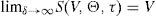
All of the above allows us to establish the following theorem.Theorem Suppose S(V,τ)>0, and let φδ≡ℜ+, φψ1≡(ψˆ1,∞), φτ1≡(τ, ∞). Consider any sequence α–β–γ, where α is chosen in φα, and define φβ|αas the subset of φβfor which S(V,Θ,τ)=S(V,τ) reaches a solution for at least one γ∈φγ, given α. For any Δ, φβ|αis a non empty set. Moreover, for any α∈φα, and β∈φβ|α, there is only one γ∈φγsuch that S(V,Θ,τ)=S(V,τ). See Appendix A. ΘF≠∅ if and only if S(V,τ)>0. This holds given lemma and theorem above.
The theorem asserts that, whenever S(V,τ)>0, a feasible RC with any arbitrary capital structure can be generated, and also describes how can it be constructed. Although this feasible Θ is not unique for a given Δ, and there is actually an infinite number of elements in ΘF|Δ, not everything is possible. Choosing one element in ΘF|Δ could be seen as a matter of priority. Take for instance the sequence τ1–δ–ψ1. The maturity of the first payment, τ1, is freely chosen in the interval (τ,∞). However, this election restricts the range of the dividend rates, δ, that can be selected in [0,∞), and the election of the dividend rate in the restricted interval finally determines a unique first debt payment, ψ1, in (ψˆ1,∞). On the other hand, Corollary 1 implies that refinancing is feasible under the same conditions that it is feasible to issue new equity to pay the debt. Note also that S(V,t)>0 ∀t<τ given limited liability, what would allow the firm to refinance for any t<τ.
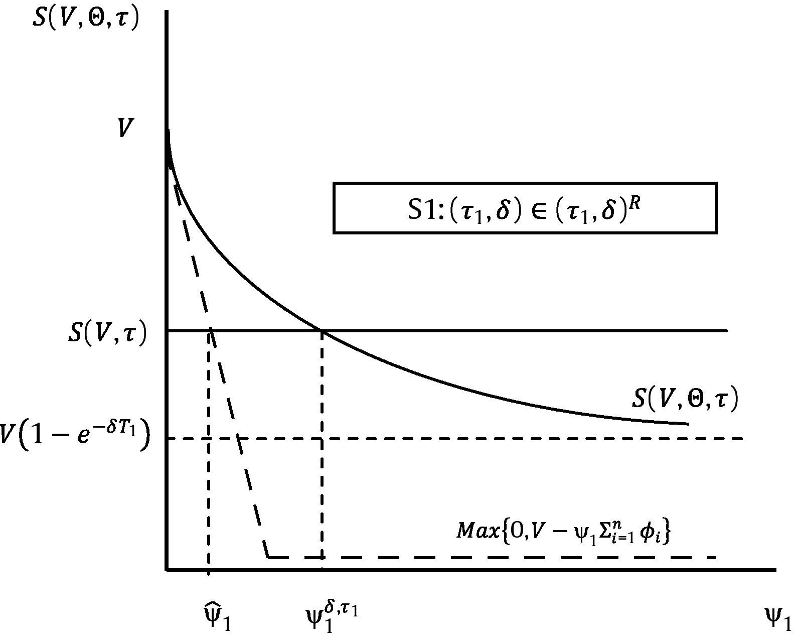
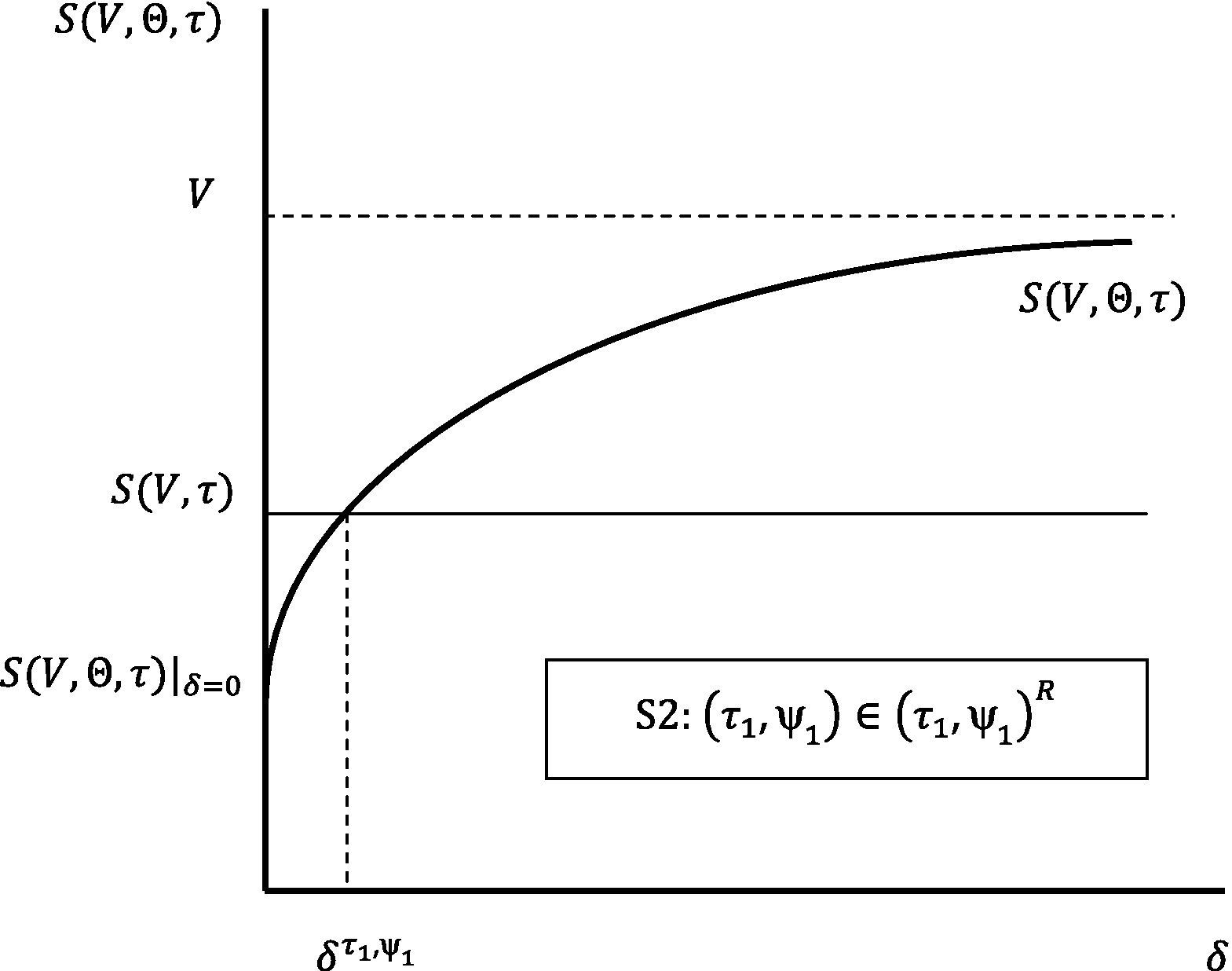
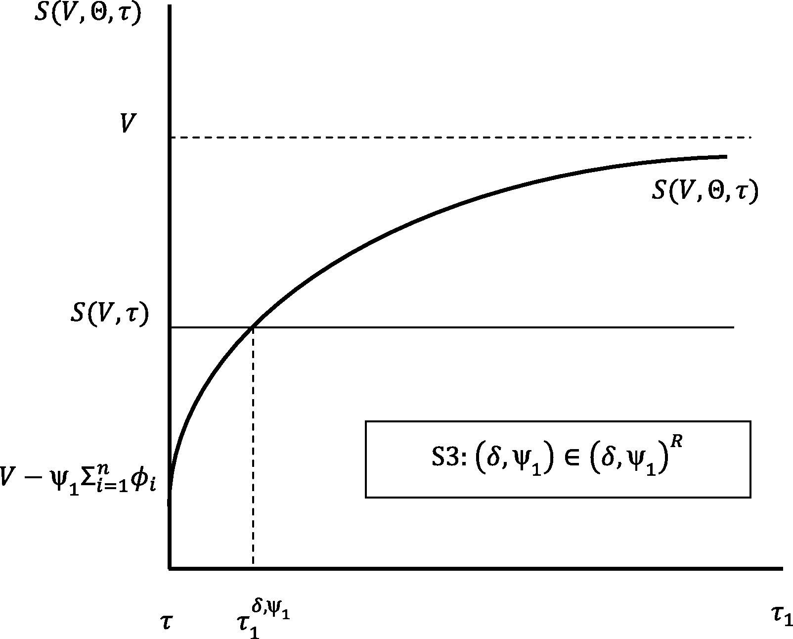
We end this section with an additional corollary which establishes a joint restriction on the possible values of (τ1,δ), (τ1,ψ1), and (δ,ψ1), that need to be satisfied in any refinancing contract. This corollary follows directly from the proof of the theorem.Corollary 2 Consider the following scenarios: S1: (τ1,δ)∈(τ1,δ)R, where (τ1, δ)R≡(τ1, δ)∈φτ1×φδ|δT1<ln[V/F(V, τ)]; S2: (τ1,ψ1)∈(τ1,ψ1)R, where (τ1, ψ1)R≡(τ1, ψ1)∈φτ1×φψ1|S(V, Θ, τ)|δ=0≤S(V, τ); S3: (δ,ψ1)∈(δ,ψ1)R, where (δ, ψ1)R≡(δ, ψ1)∈φδ×φψ1.
For any scenario (α,β)∈(α,β)R, there is one, and only one γ∈φγ, such that the RC generated in this way is feasible.
ProofSee Appendix A.
Figs. 1–3 reflect the arguments in Corollary 2 for the three possible scenarios: S1, S2 and S3.
∈(τ1,δ)R there exists one, and only one ψ1∈φψ1, such that the RC generated in this way is feasible.")
∈(τ1,ψ1)R there exists one, and only one δ∈φδ, such that the RC generated in this way is feasible.")
∈(δ, ψ1)R there exists one, and only one τ1∈φτ1, such that the RC generated in this way is feasible.")
The fact that any possible debt structure can be chosen, joint with the freedom to select any sequence α–β–γ, gives the RC the possibility to be as “imaginative” as one may desire. We may, nevertheless, describe how to design two types of contracts that are commonly used in practice: loans which are paid in equal monthly installments, and coupon bonds.
In our notation, the type of loan described can be represented by a vector Δ, where n is equal to the number of years times 12, and Φ as well as Λ are given by a vector of dimension n with all elements equal to 1. In order to guarantee that we obtain monthly payments, we may start by choosing τ1. If we fix τ equal to zero, and if we assume that μ and σ are in annual terms, then τ1 equal to 1/12 generates the monthly payments desired. Corollary 2 finally ensures that for any δ lower that 12×ln[V/F(V,0)] we will be able to find a ψ1 value in the interval (F(V,0)/n,∞), such that the resulting contract allows the firm to refinance; a contract that implies equal monthly installments.
A coupon bond will require a little bit more of elaboration. Clearly, this way to refinance needs the debt principal to be equal to F(V,τ). If coupons are paid annually, then n will be the number of years, and Λ will be a vector of ones of dimension n. Φ this time will be given by a vector of dimension n, with all elements equal to 1 but the element n, which will be equal to (1+p). Consider again period τ equals zero, and choose τ1=1 to guarantee annual payments. Again we can use Corollary 2 to ensure that there exists a ψ1 in the interval (F(V,0)/(n+p),∞) that allows the firm to refinance for any δ lower than ln[V/F(V,0)]. According to Φ, we will have equal coupon payments between periods 1 and n−1, and the payment of coupon plus ψ1p at the final date n. But we need a pair of values (ψ1,p) such that the equality ψ1p=F(V,0) holds. As a first step we may prove that such a pair exists. Note that this equality, joint with restriction ψ1>F(V,0)/(n+p), leads to ψ1n>0. In short, equity holders could pay F(V,0) at τ=0, or defer this payment to a future period. Condition ψ1n>0 simply says that at least a coupon payment is needed in order to charge the interests that debt holders will require for this deferment. The problem is that, in general, ψ1p will not be equal to F(V,0). We could however use a tivial “trial and error” method to find these two values.5 At the end we will have designed a coupon bond that allows the firm to refinance.
We next analyze the specific cases of n=1 and n=2. These will be useful to provide the basic implications of the refinancing strategy.
3Particular cases3.1n=1Although any possible initial debt structure could be considered, we will assume in this case that n remains constant along time. This means that a single zero coupon bond, with nominal ψ and maturity at τ, is replaced by a single zero coupon bond, with some nominal ψ1 and some maturity τ1>τ, whenever S(V,τ)>0. In order to show that a feasible RC exists, we need to describe how S(V,Θ,τ) is to be valued. Specifically, we need to find the equity value at τ, when the corporate debt consists in the payment of ψ1 at τ1>τ, and the dividend rate is δ, that is, S(V,Θ,τ) for Θ≡(δ,ψ1,τ1).
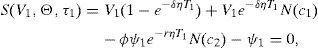
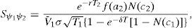
S(V,Θ,τ) has two sources of value. On one hand the value associated to the dividends that will be received between τ and τ1, D(V,τ). On the other hand the option value, O(V,τ), that comes from the possibility of acquiring the firm at τ1 by paying ψ1. Applying risk neutral valuation we find that
and6whereFinally,where it is straightforward to check that Assumption B actually holds.7

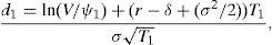

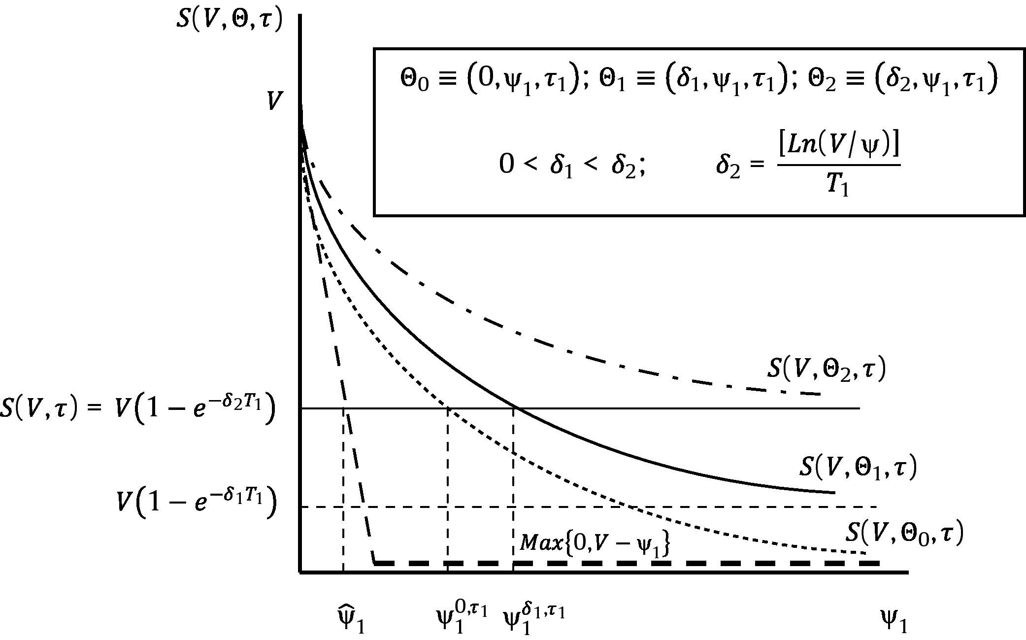
Fig. 4 describes two of the six alternative ways to design a RC with n=1: those associated to the sequences τ1–δ–ψ1 and τ1–ψ1–δ, respectively.8

Consider first τ1–δ–ψ1. In principle, any dividend rate between zero and infinity would be feasible in a RC. However, for a given maturity τ1 strictly greater than the refinancing period τ, the set of possible dividend rates reduces to the interval [0,δ2). We may say that the higher the debt maturity, the lower the dividend rate that debt holders will be willing to accept to refinance existing debt. Now let us assume that a debt maturity has been chosen. Fig. 4 makes clear that the higher δ, the higher the debt payment, or in other words, the higher the yield that debt holders will charge to the firm to refinance its debt.
Sequence τ1–ψ1–δ can also be analyzed using Fig. 4. In this specific case of n=1, it is clear that ψˆ1=ψ. Nevertheless, any debt maturity τ1 strictly greater than the refinancing moment τ will lead to a strictly positive yield reflected in a higher ψ1. For a fixed maturity we observe on the other hand that the higher the yield charged to equity holders, that is, the higher ψ1, the higher also the dividend rate. In short, equity holders demand a higher dividend rate as compensation for bearing a higher interest rate.
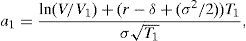
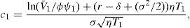
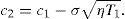
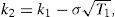
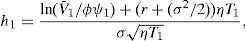
An interesting aspect is that, in fact, the credit spread (C.S) on corporate debt that results from refinancing will depend on the specific RC chosen in the feasible set; a feasible set that at the same time depends on the current firm value, the current nominal debt, the firm return volatility, and the risk free interest rate. We know that for any element Θ of this set, the new equity value, S(V,Θ,τ), equals the previous one, S(V,τ). This can be expressed as V−ψ1e−RT1=V−ψ, where R is the interest rate associated to the new corporate debt. Then it is straightforward to show that
Although the dividend rate does not explicitly appear in the expression above, it does through its influence on ψ1 and T1.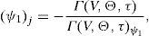
Given the firm characteristics and the risk free rate, that is, given a vector (V,ψ,σ,r), the C.S will be a function of the specific contract chosen, which we represent by a vector (δ,ψ1,τ1). We have seen however that only two of these three elements are “freely” chosen. Consider for instance (τ1,δ) are selected according to the restriction imposed by Corollary 2 (S1), then the credit spread will be a function of (V,ψ,σ,r,δ,τ1), with δT1<ln(V/ψ). In order to make some comparative statics with respect to the C.S, we need to derive how ψ1 depends on these variables and parameters. Let us define Γ(V,Θ,τ)=S(V,Θ,τ)−S(V,τ); then, Θ belongs to the feasible set if and only if Γ(V,Θ,τ)=0, and the derivative of ψ1 with respect to variable or parameter j will be given by
what leads to (ψ1)V<0, (ψ1)ψ>0, (ψ1)σ>0, (ψ1)r>0, (ψ1)δ>0, (ψ1)τ1>0.9 We may now describe the dependence of the C.S on the firm value and on the nominal debt to be refinanced.A higher leverage ratio (a lower V or a higher ψ), means a higher credit risk, and the result is a higher C.S faced by the firm to refinance.
On the other hand,
It is also reasonable to observe that the higher the firm risk, the higher the credit spread on the firm debt.
The credit spread shows however to be independent of the risk free interest rate:
This result is not in contradiction with Merton's (1974) prediction of an inverse relation between the credit spread of a zero coupon bond and the risk free rate. On the contrary, it extends the analysis to what will tend to happen in the medium and long run. To see this, assume an increase in the risk free rate at current period t. According to the arguments in Merton (1974) we will see an immediate fall in the credit spread at t; however, previous arguments imply that this effect will only persist up to the refinancing date τ. In addition, the nominal of the new debt, ψ1, will be higher the higher the risk free rate. As a consequence, the credit risk premium that the firm will assume at τ1 to refinance ψ1, will tend to be higher the higher the risk free rate at τ, given that this premium is an increasing function of the initial debt. We then conclude that under the assumption of debt refinancing with n=1, an increase in the risk free rate reduces the credit spread in the very short run, has no effect in the medium run, and turns to have a positive effect in the long run. There is evidence at least of the first prediction. In fact, Longstaff and Schwartz (1995) show empirically that credit spreads exhibit an inverse relation with respect to changes in the interest rate on Government Bonds. It would be interesting to check whether the predictions for the medium and long run also hold.
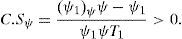
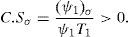
The dependence of the credit spread on the dividend rate is described by
A higher dividend rate implies a lower expected firm value growth and a higher default probability, what leads to a higher credit spread.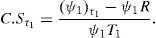
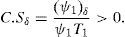
Finally,

While an analytical solution for the sign of C.Sτ1 cannot be provided, it has shown to be positive in all simulations performed. Again, this result may seem inconsistent with the results in Merton (1974). It must be pointed out the substantial difference in the analysis of the time dependence followed by Merton and the one we drive here (not only the inclusion of a dividend rate). In fact, he sets the so-called “quasi debt-to-firm value ratio” constant. In order to keep this ratio equal to a fixed q for a given firm value and interest rate, ψ1 should be determined as qVerT. In our case, however, we impose that the implied ψ1 value is consistent with a feasible RC, what makes the ratio q to move from values below 1 to values above 1 for different maturities.10
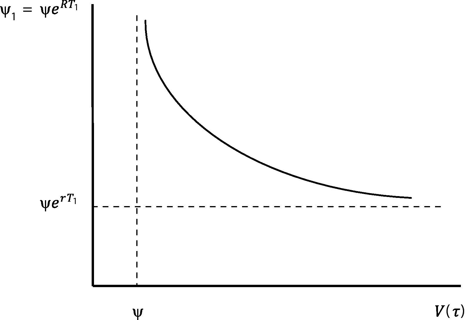
The fact that a firm chooses to refinance its debt has also several implications in terms of the future evolution of credit ratings and credit spreads. To start with, we may represent the new nominal debt payment that results from refinancing at τ as a function of the firm value. This is show in Fig. 5. As the firm value tends to the default point ψ, the new nominal payment (and the credit spread that the firm has to face to refinance) tends to infinity. As the firm value tends to infinity on the other hand, the new payment tends to the previous payment capitalized at the risk free interest rate.11
.")
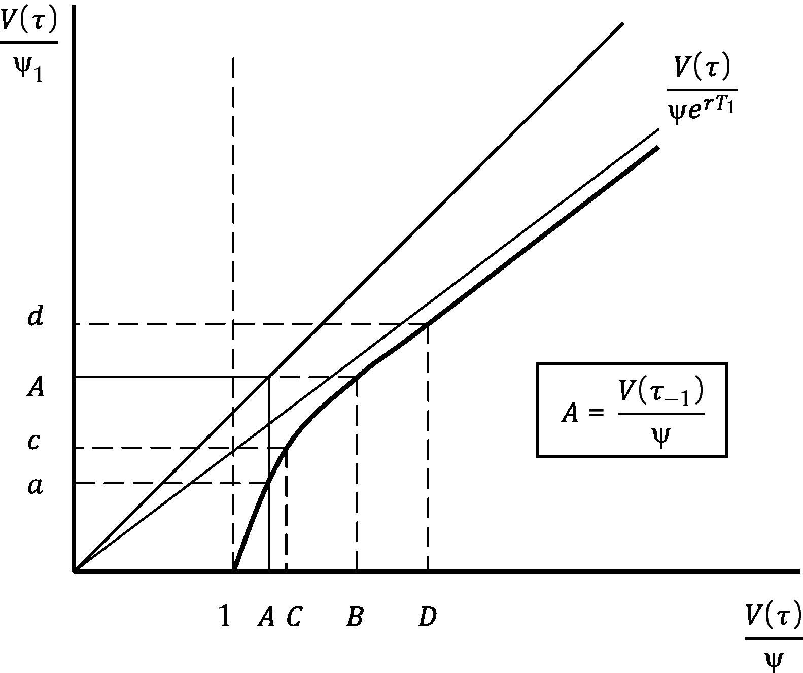
Let us now assume that the credit rating of the firm is measured at any time the firm refinances, as the ratio current firm value to new nominal debt. Fig. 6 follows directly from Fig. 5, and represents the credit rating at τ, V(τ)/ψ1, as a function of the ratio V(τ)/ψ. Let A=V(τ−1)/ψ be the credit rating of the firm at issuance of ψ. Then, if the firm value stays constant between τ−1 and τ, the credit rating falls to a. The fact that the firm refinances makes possible to observe a downgrade in the credit rating of the firm even if it does not lose market value and, as Fig. 6 indicates, even with a strictly positive growth (point C). In order to keep its credit rating a firm value growth large enough (point B), has to take place. In summary, any ratio V(τ)/ψ lower that B will be followed by a downgrade, while any value of this ratio above B will lead to an upgrade. Note also that deviations from B will have a different impact on the credit rating depending on whether this deviation is positive or negative. A negative deviation will have a higher effect in absolute terms than an equivalent positive deviation. Debt refinancing therefore is expected to generate stronger downgrades than upgrades.
3.2n=2/ψ1 as a function of V(τ)/ψ.")
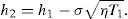
We have analyzed the case in which the firm always maintains a single zero coupon bond as corporate debt. The main implications derived from assuming that the firm refinances its debt in terms of credit ratings and credit spreads appear in this simple case. Exploring the situation in which the firm always refinances with n=2 is interesting however for several reasons. First, it can be seen as a simplification to short and long term debt, what better represents the debt structure of a firm. Second, it incorporates the fact that equity holders do not only care about the debt that currently matures at the time of deciding whether or not satisfying it, but also about all future debt remaining. This makes for instance the current bankruptcy-triggering firm value to diverge from the current nominal debt payment, something that does not happen with n=1. Proposition 1 ensures that at any time the firm has to satisfy a debt payment, refinancing with n=2 is feasible.Proposition 1 B1–B3 hold for n=2, making a refinancing contract with n=2 feasible whenever S(V,τ)>0. See Appendix A.
Proposition 1 does not assume any specific initial debt structure. However, we may think in a model in which the firm maintains a stable corporate debt structure with short and long term debt, keeping the ratio short term debt/long term debt, and the time spread between them, constant. This stable corporate debt structure translates into a vector Δ≡(n,Φ,Λ), where n=2, Φ=(1,ϕ) and Λ=(1,η). Assume again that the firm does not pay dividends. As a result, it is always possible to consider that the firm refinances not only under a constant Δ (as stated in the theorem), but also with some fixed T1 (see Corollary 2, S1). The following proposition implies that the effect of debt refinancing on the evolution of the credit rating of the firm described for n=1, also applies in this case.Proposition 2 LetV¯andV¯1denote the bankruptcy-triggering firm value at τ and τ1respectively. Then, V¯1is a strictly decreasing and strictly convex function in V(τ), withlimV(τ)→V¯V¯1=∞andlimV(τ)→∞V¯1=V¯erT1. See Appendix A.
The shape of V¯1 as a function of V(τ) will be therefore analogous to the one we found for ψ1 with respect to V(τ) under n=1. The credit rating at τ will be now described by the ratio V(τ)/V¯1, and the same analysis we made for V(τ)/ψ1 applies in this case. Refinancing makes V¯1 to be the new bankruptcy-triggering firm value, a critical threshold that will evolve over time as the firm refinances its debt repeatedly. Although no explicit solution for it can be provided, it can be shown to belong to the same range in which KMV typically finds to be the default point.Proposition 3 Let ψ1and ψ2be the new short and long term debt resulting from refinancing at τ, and let T be the time spread between these payments. Then, for anyσ∈(0,∞), V¯1∈(ψ1,ψ1+ψ2e−rT). Moreover, limσ→0V¯1=ψ1+ψ2e−rT and limσ→∞V¯1=ψ1. See Appendix A.
With a database of over 100,000 company-years and over 2000 incidents of default or bankruptcy, KMV has found that firms generally default when the firm value lies somewhere between short term debt and total debt in nominal terms.12 Clearly, V¯1∈(ψ1,ψ1+ψ2e−rT) implies that V¯1∈(ψ1,ψ1+ψ2).
4ConclusionsRefinancing existing debt seems to be one of the most important, if not the first, reason to issue new debt. We investigate the long run effects of this extended practice on credit ratings and credit spreads. Debt refinancing generates systematic rating downgrades unless a minimum firm value growth is observed. Deviations from this growth path imply asymmetric results. A lower firm value growth generates downgrades and a higher firm value growth upgrades as expected. However, downgrades will tend to be higher in absolute terms. Finally, the risk free rate will have a negative effect over the credit spreads in the short run, a null effect in the medium run, and a positive effect in the long run.
Forte acknowledges financial support from MEC Grant Ref: AP2000-1327 and Banco Sabadell. Peña acknowledges financial support from MEC grants PB98-0030 and BEC2002-00279, and MCI grant ECO2009-12551. Preliminary versions of this paper have been presented with the title “Debt Financing and Default Probabilities” at the IX Foro de Finanzas (Pamplona), and with the title “The Design of Refinancing Contracts” at LACEA 2002. The authors appreciate helpful comments from Carmen Ansotegui and an anonymous referee. The usual disclaimers apply.
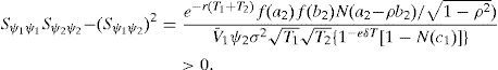
S(V,Θ,τ) is what equity holders get after signing Θ, therefore, they will be willing to sign if and only if S(V,Θ,τ)≥S(V,τ). F(V,Θ,τ) is what debt holders have after signing Θ, therefore, they will be willing to sign if and only if F(V,Θ,τ)≥F(V,τ). At the same time S(V,Θ,τ)+F(V,Θ,τ)=S(V,τ)+F(V,τ)=V. S(V,Θ,τ)=S(V,τ) implies that F(V,Θ,τ)=F(V,τ) and Θ∈ΘF. On the other hand Θ∈ΘF implies S(V,Θ,τ)≥S(V,τ). Suppose S(V,Θ,τ)>S(V,τ), then F(V,Θ,τ)<F(V,τ) and Θ∉ΘF, what is a contradiction, proving the first argument of the lemma. Finally, S(V,Θ,τ)>0 ∀Θ|τ1>τ, implying S(V,τ)>0 as a necessary condition for a feasible Θ to exist.1313 Limited liability makes S(V,Θ,τ)>0 when no payment has to be currently satisfied.
We have six possible sequences α–β–γ. Let us analyze each one of them:Case 1τ1–δ–ψ1 Given τ1∈φτ1, S(V,Θ,τ) is CSD (ψ1), with limψ1→ψˆ1S(V,Θ,τ)>S(V,τ) ∀δ∈φδ, and limψ1→∞S(V,Θ,τ)=V(1−e−δT1). Therefore, S(V,Θ,τ)=S(V,τ) reaches a solution for at least one ψ1∈φψ1, if and only if V(1−e−δT1)<S(V, τ), if and only if δ<ln[V/F(V, τ)]/T1. As a result, φδ|τ1≡[0, ln[V/F(V, τ)]/T1)≠∅. Because S(V,Θ,τ) is CSD (ψ1), we finally have that for any τ1∈φτ1, and δ∈φδ|τ1, there is a unique ψ1∈φψ1 such that S(V,Θ,τ)=S(V,τ). Given τ1∈φτ1, S(V,Θ,τ) is CSI (δ), with limδ→∞S(V, Θ, τ)=V ∀ψ1∈φψ1. Therefore, S(V,Θ,τ)=S(V,τ) reaches a solution for at least one δ∈φδ, if and only if S(V, Θ, τ)|δ=0≤S(V, τ), if and only if ψ1≥ψ10,τ1, where ψ10,τ1>ψˆ1 is the ψ1 value such that S(V, Θ, τ)|δ=0=S(V, τ).1414 B1 implies that ψ10,τ1 exists and is unique, and joint with B2 also implies that ψ10,τ1>ψˆ1. Given δ∈φδ, S(V,Θ,τ) is CSD (ψ1), with limψ1→ψˆ1S(V,Θ,τ)>S(V,τ) ∀τ1∈φτ1, and limψ1→∞S(V,Θ,τ)=V(1−e−δT1). Therefore, S(V,Θ,τ)=S(V,τ) reaches a solution for at least one ψ1∈φψ1, if and only if V(1−e−δT1)<S(V, τ), if and only if τ1<τ+ln[V/F(V,τ)]/δ. As a result, φτ1|δ≡(τ, τ+ln[V/F(V, τ)]/δ)≠∅. Because S(V,Θ,τ) is CSD (ψ1), we finally have that for any δ∈φδ, and τ1∈φτ1|δ, there is a unique ψ1∈φψ1 such that S(V,Θ,τ)=S(V,τ). Given δ∈φδ, S(V,Θ,τ) is CSI (τ1), with limτ1→τS(V,Θ,τ)=V−ψ1∑i=1nϕi<S(V,τ) ∀ψ1∈φψ1, and limτ1→∞S(V,Θ,τ)=V. As a result, φψ1|δ≡φψ1≠∅. Because S(V,Θ,τ) is CSI (τ1), we finally have that for any (δ, ψ1)∈φδ×φψ1, there is a unique τ1∈φτ1 such that S(V,Θ,τ)=S(V,τ). Given ψ1∈φψ1, S(V,Θ,τ) is CSI (δ), with limδ→∞S(V, Θ, τ)=V ∀τ1∈φτ1. Therefore, S(V,Θ,τ)=S(V,τ) reaches a solution for at least one δ∈φδ, if and only if S(V, Θ, τ)|δ=0≤S(V, τ), if and only if τ1≤τ10,ψ1, where τ10,ψ1>τ is the τ1 value such that S(V, Θ, τ)|δ=0=S(V, τ).1515 B2 implies that τ10,ψ1 exists and is unique. B2 also implies that τ10,ψ1>τ. Given ψ1∈φψ1, S(V,Θ,τ) is CSI (τ1), with limτ1→τS(V,Θ,τ)=V−ψ1∑i=1nϕi<S(V,τ) ∀δ∈φδ, and limτ1→∞S(V,Θ,τ)=V. As a result, φδ|ψ1≡φδ≠∅. Because S(V,Θ,τ) is CSI (τ1), we finally have that for any (ψ1, δ)∈φψ1×φδ, there is a unique τ1∈φτ1 such that S(V,Θ,τ)=S(V,τ).
This holds for S1, S2 and S3, given the proof of the theorem for cases 1 and 3, 2 and 5, and 4 and 6, respectively.
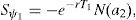
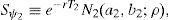
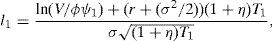
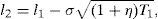
Let T1=τ1−τ and T2=τ2−τ. Following the restriction imposed in Section 2 we will express ψ2 as ϕψ1, and T2 as (1+η)T1. The equity value is given in this case by
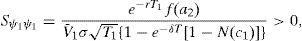
where N2(a,b;ρ) represents the standard bivariate normal distribution function, with integration limits a and b, and correlation coefficient ρ. In addition,where V¯1 is the firm value that satisfieswithS(V,Θ,τ) is then a continuous function in ψ1, withThis, joint withproves that Assumption B1 holds.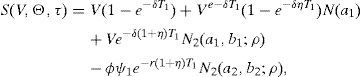


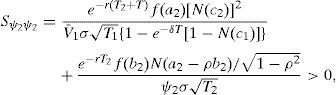
At the same time S(V,Θ,τ) is a continuous function in τ1, with
proving that Assumption B2 also holds.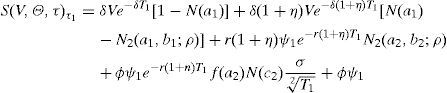

Finally, S(V,Θ,τ) is a continuous function in δ, with
implying that Assumption B3 is equally satisfied.1616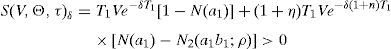
A more detailed description of the steps followed in this proof is available upon request.
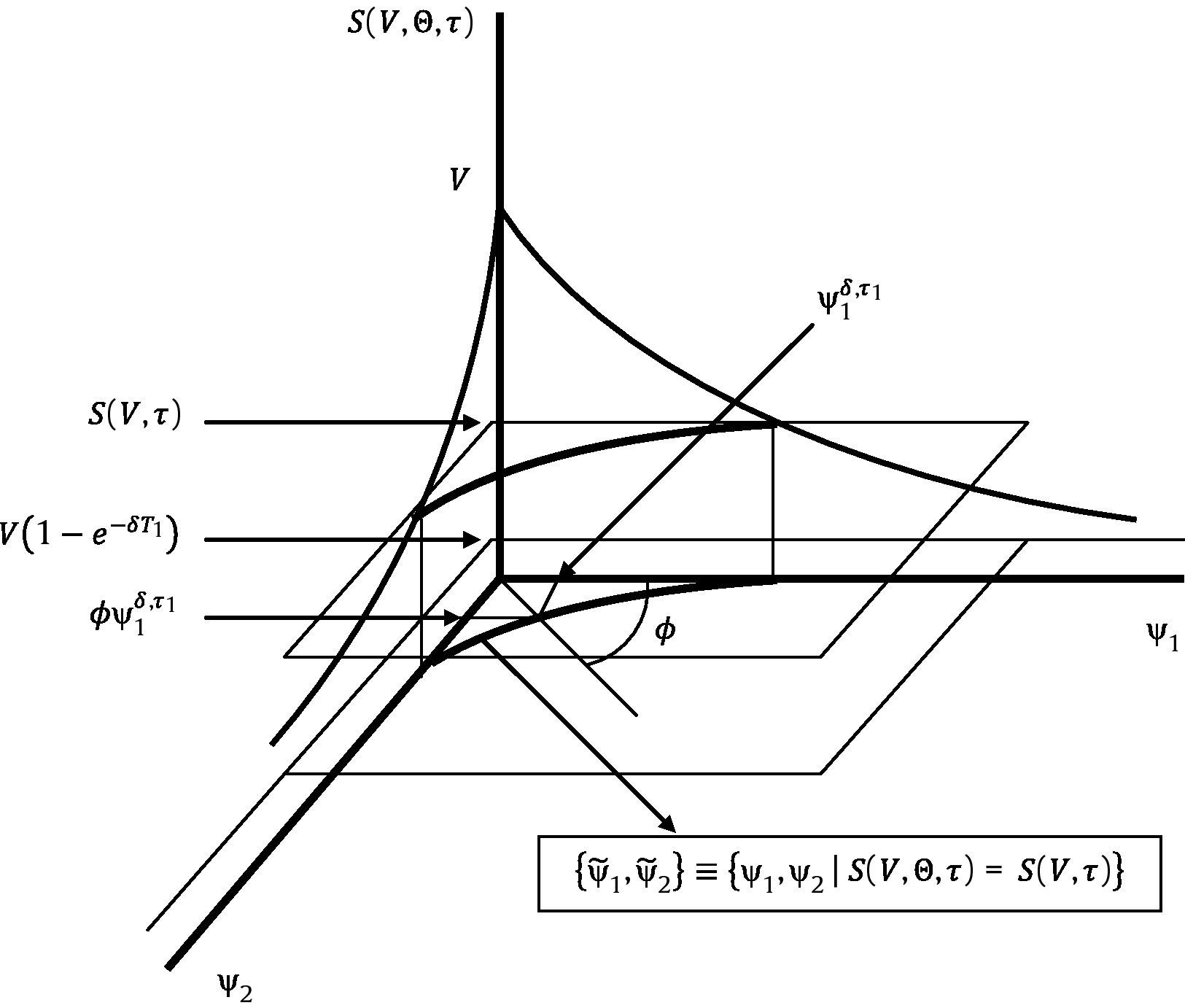
It is possible to analyze graphically case 1 for n=2. Let denote S(V,Θ,τ) simply as S, and let show that S is strictly convex in (ψ1,ψ2), where we do not impose the restriction ψ2=ϕψ1.
The strict convexity of S, joint with S|(ψ1,ψ2)=(0,0)=V, and lim(ψ1,ψ2)→(∞,∞)S=V(1−e−δT1), leads to Fig. 7.

Let ψ be the debt payment to be satisfied at τ. Then
whereand S(V,τ)>0 ∀V>V¯, being V¯ the implicit solution to S(V¯,τ)=0.
On the other hand,
whereand V¯1 is the implicit solution towithIf we define θ=V¯1/ψ1, then previous expression can be written aswhere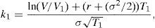


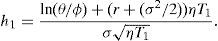

The result is that θ is a constant, that is, θ will not depend on the firm value at τ (although V¯1 and ψ1 will). Note also that θ=V¯/ψ. We can express condition Γ(V,Θ,τ)=S(V,Θ,τ)−S(V,τ)=0 as
where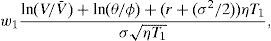

This condition implies that as V tends to V¯,V¯1, tends to infinity. At the same time, limV→∞V¯1=V¯erT1.1717 Note that this implies that limV→∞ψ1=ψerT1 and limV→∞ϕψ1=ϕψerT1, that is, as the default risk tends to zero, new debt payments tend to current payments capitalized at the risk free interest rate.

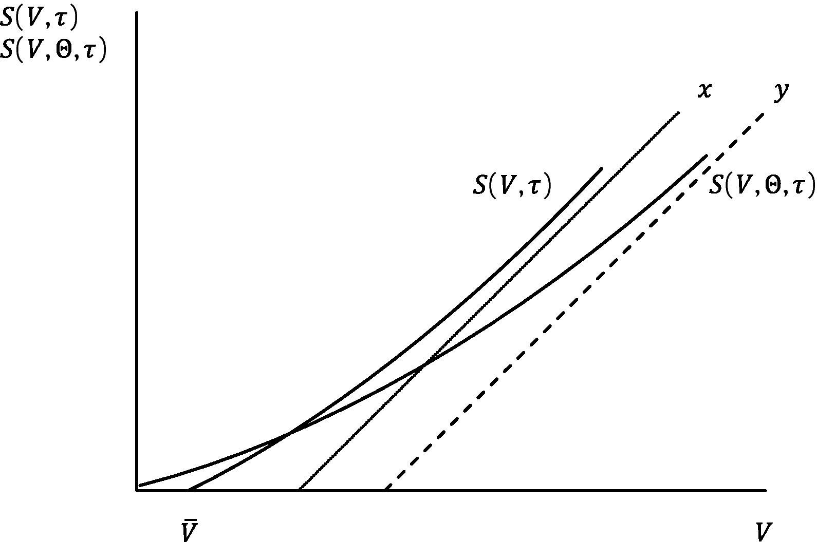
Fig. 8 represents S(V,τ) and S(V,Θ,τ) as a function of V.1818 x=V−V¯(ϕ/θ)e−rηT1−V¯(1/θ) and y=V−V¯1(ϕ/θ)e−r(1+η)T1−V¯1(1/θ)e−rT1. V¯(ϕ/θ)e−rηT1+V¯(1/θ)<V¯1(ϕ/θ)e−r(1+η)T1+V¯1(1/θ)e−rT1 given V¯1>V¯erT1.
 and S(V,Θ,τ) as a function of V for n=2.")
Let
wherethen, V¯1≡V|Z(V)=0.
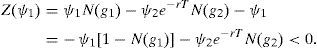
Suppose first σ∈(0,∞) and V=ψ1; then
This, joint with ZV=N(g1)>0, implies that V¯1>ψ1 ∀σ∈(0,∞). We have that limσ→∞N(g1)=1 and limσ→∞N(g2)=0, therefore, limσ→∞Z(V)=V−ψ1=0⇔V=ψ1, proving limσ→∞V¯1=ψ1.
On the other hand, consider V=ψ1+ψ2e−rT; then

limσ→0Z(ψ1+ψ2e−rT)=0 because limσ→0N(g1|V=ψ1+ψ2e−rT)=limσ→0N(g2|V=ψ1+ψ2e−rT)=1. As a result, V¯1=ψ1+ψ2e−rT in this limit case. Given that Zσ>0 we also have that Z(ψ1+ψ2e−rT)>0 ∀σ∈(0,∞). This, joint again with ZV=N(g1)>0, implies V¯1<ψ1+ψ2e−rT ∀σ∈(0,∞), and concludes the proof.

