


In this paper we approach the inflation expectations and the real interest rate by using the information contained in the yield curve. We decompose nominal interest rates into real risk-free rates, inflation expectations and risk premia using an affine model that takes as factors the observed inflation rate and the parameters generated in the zero yield curve estimation. Under this approach we could obtain a measure of inflation expectations free of any risk premia. Moreover in our estimation we avoid imposing arbitrary restrictions as is mandatory under other methodologies based on unobserved components.
The empirical exercise has been applied to an economy – like the Spanish one during the 90s – with an important convergence process and a change in the monetary policy regime. The results suggest that the evolution of inflation expectations has been smoother than was expected.
Inflation expectations and real risk-free rate are two variables that are not observable although their evolution affects the nominal interest rates. In fact, nominal interest rates can be decomposed, from a theoretical perspective, into three components: real risk-free rates, inflation expectations and risk premia. Disentangling which component is the main driver of some of the changes seen in nominal interest rates is often crucial in several different realms such as bond pricing, the analysis of investment or other expenditure decisions made by firms or households or in the process of monetary policy decision-making. Unfortunately, however, the above-mentioned components are not directly observable and the literature only proposes partial solutions to obtain this decomposition.
The most common approach consists in taking inflation expectation as the inflation finally observed and subtracting this ex-post inflation rate from nominal interest rates to obtain an estimate of real risk-free rates. This implies assuming that there is no risk premium and also that agents are able to perfectly foresee the inflation rate. These assumptions are most likely to be only slightly restrictive in reasonably stable economies where the variability of prices is small. However, in other cases the risk premia or the inflation expectations errors could be significant. Moreover, if the economy exhibits some convergence process or if the central bank modifies its monetary policy strategy it seems natural to expect significant variations in risk premia and/or (rational) important mistakes when forecasting inflation. This is for instance the case of Spain and several other European countries involved in EMU creation where uncertainty over convergence finally achieved and the introduction of an inflation targeting for the Banco de España could have originated fluctuations on these variables. Another well known example of sharp modifications in the monetary policy stance was the beginning of the Volcker period as governor of the Board of the Federal Reserve. In those environments, ex-post real interest rates could provide a misleading approach to the actual behavior of real risk-free rates and inflation expectations could not be properly approximated by its ex-post values.
An alternative to ex-post real rates consists in using the return on inflation-indexed bonds to approach real rates, whereas inflation expectations are estimated as the difference with respect to their nominal reference. However, these bonds are not traded in many countries or have been introduced only recently. In addition, although this alternative provides an intuitive estimation of real rates, it does not consider the risk premia and thus provides a biased estimation of both real risk-free rates and inflation expectations (see Evans, 1998), a bias that in some circumstances – let us think of the Great Moderation process (see Summers, 2005), can hardly be negligible.
Against this background, this paper proposes a methodology to decompose nominal interest rates into its three components from an affine model of the nominal term structure. This methodology is related to the macro-finance literature in which authors such as Diebold et al. (2006), Diebold et al. (2005), Carriero et al. (2006), and Ang et al. (2008) (ABW) incorporate macro-determinants into a multi-factor yield curve model with non-arbitrage opportunities. Our decomposition departs from previous approaches by extracting the risk premia from the difference between the nominal term structure and a notional term structure where the price of risk is set equal to zero.
We also propose a new affine model where interest rates are affine relative to a vector of factors that includes inflation rates and exogenously determined factors based on the Nelson–Siegel exponential components of the yield curve (Nelson and Siegel, 1987) in a similar vein to Carriero et al. (2006) and Diebold and Li (2006). Moreover, in our case we include the condition of non-arbitrage opportunities along the yield curve as well as taking into account the risk-aversion. Taking these two conditions together allows us to decompose nominal interest rates as the sum of real risk-free interest rates, expected inflation and the risk premium. We therefore depart from Dai and Singleton (2000), Laubach and Williams (2003), and ABW (2008), who consider latent components, which they endogenously estimate. The latent component methodology depends heavily on the initial conditions and the arbitrary selection of some maturities that have to be observed without error as well as some ad-hoc restrictions on the parameters (Kim and Orphanides, 2005). Our proposal supposes a less restrictive approach and the results seem to be more robust.
This model and decomposition methodology are applied to the Spanish nominal interest rates during the nominal convergence period that led the Spanish economy to be one of the eleven first members of the Economic and Monetary Union. The decomposition exercise shows a decline in Spanish real risk-free interest rates during the nineties of an order close to 3pp, a figure significantly lower than the estimations with other methodologies. In fact, Blanco and Restoy (2011) highlights that traditional approaches that produce much higher declines in real risk-free rate, are not compatible with the observed evolution of Spanish macroeconomic figures (such as GDP growth rate or employment rate) and the increase experienced by some asset prices, such as the case of stock or house prices. Moreover, the results show that, during some episodes, long-run expected inflation rates were systematically higher than ex-post actual inflation rates. This finding could very likely be reflecting the uncertainties surrounding the Spanish success in fulfilling the Maastrich criteria on time. In fact, risk premia upturns coincide with the shifts in inflation expectations. Thus changes in inflation expectations and inflation risk premia account for a substantial part of the decrease in nominal interest rates during the convergence process.
The rest of the paper is structured into three further sections. In Section 2, we derive the decomposition of nominal interest rates and in Section 3 we describe the main results for the Spanish economy. Finally, Section 4 concludes.
2Modeling interest rates2.1The affine modelAs stated by Piazzesi (2009), affine term structure models allow the risk premium to be separated from expectations about future interest rates. These models have been widely used in the financial literature to price fixed-income assets since the seminal works of Vasicek (1977) and Cox et al. (1985). Including inflation in the specification of the model, as in ABW (2008) and in Carriero et al. (2006), will also make it possible to jointly estimate inflation expectations and real interest rates.
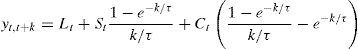
An affine model assumes that interest rates can be explained as a linear function of certain factors,
where yt,t+k is the nominal interest rate in period t with term k, Xt is a vector of factors, Ak and B′k are coefficients and ut,t+k represents the measurement error. Changes in interest rates across time will be the outcome of changes in the factors, whereas differences in the term structure will be driven by the coefficients Ak and B′k applied.
There is extensive evidence on the predictability of interest rates (see Diebold and Li, 2006), and this feature is usually included in the affine model by assuming that Xt factors follow a VAR structure (in the same vein as Diebold et al., 2006),
where μ is a vector of the constant drifts in the affine variables Xt, Σ is the variance–covariance matrix of the noise term and Φ is a matrix of the autoregressive coefficients. The VAR model accounts for the observed predictability in the interest rates but allows, at the same time, some degree of uncertainty in the future values of interest rates, represented by the noise vector ¿t that follows a standard i.i.d. Gaussian normal distribution. In order to avoid identification problems we will impose matrix Σ to be diagonal in Eq. (2), so relationships between factors Xt will be reflected by coefficients of matrix Φ rather than shocks.1
In order to avoid arbitrage opportunities, the values of parameters Ak and B′k of Eq. (1) should be restricted according to Eq. (3),
The left hand-side of Eq. (3) represents the valuation of a zero-coupon bond with maturity in k+1 that under the non-arbitrage condition should be equivalent to the expected value one period ahead of the same bond with maturity k discounted with the short-term interest rate. As can be seen in Annex 1, solving forward Eq. (3) implies a recursive form for the Ak and B′k coefficients.
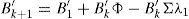
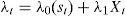
The consideration of risk-aversion in this framework implies some compensation for the uncertainty about longer maturities,2 in which the random shocks ¿t accumulate. In this respect, it is clear that the higher the variance of random shocks on VAR Eq. (2) (identified by matrix Σ), the greater the uncertainty about future values of interest rates. So, in order to compensate investors for lending money at longer terms, some risk premium related to Σ should be embedded in the nominal interest rates (see Annex 1). Coefficients that translate matrix Σ into the risk premium are called prices of risk (λt) and, following the literature, these coefficients are affine to the same factors Xt,
where λ0 is a vector and λ1 a matrix of coefficients. If λ1 is set to be equal to zero, then the risk premium will be constant, while if we leave it unrestricted, we will obtain a time-varying risk premium.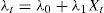
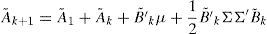
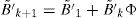
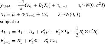
Taking together the no-arbitrage opportunities and the risk-aversion, it is possible, after some algebra (see Annex 1), to transform Eq. (2) into a recursive system of equations represented by Eqs. (5) and (6).
In Eqs. (5) and (6), the coefficients determining the interest rates with maturity in k+1 (Ak+1 and B′k+1) are the result of the aggregation of the determinants of the short-term interest rate (A1 and B′1), the difference between actual short-term interest rate and its forecasted value (reflected by Ak+B′kμ and B′kΦ terms, respectively) a compensation for risk (B′kΣλ0 and B′kΣλ1 terms, respectively), and a quadratic term consequence of the Jensen Inequality ((1/2)B′kΣΣ′B′k). As can be see, risk compensation depends on matrix Σ and the price of risk λt.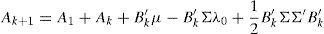
Therefore, the affine model to be estimated consists of Eqs. (1) and (2), with the coefficients of Eq. (1) being subject to restrictions 5 and 6. Differences among several affine models will be the result of the chosen Xt factors.
2.2Factor specificationWe have to consider the variables that could determine the term structure of interest rates in order to select the factors in the model of Eqs. (1) and (2). In fact, there is ample evidence in the literature that the information content of the whole term structure could be shortened to a small number of factors. The choice of these factors depends on the purpose of the exercise. One alternative is to introduce unobservable or latent components. This is the case, for example, in Duffie and Kan (1996), Duffie and Singleton (1997), Dai and Singleton (2000), Duffee (2002), and Kim and Wright (2005). These specifications allow for high degrees of flexibility in the model but the factors are hard to interpret, and the estimation is not straightforward and the results obtained could be quite unstable.
Other approaches, based on certain macroeconomic factors (see Ang et al., 2006, Dewachter and Lyrio, 2006, or Dewachter et al., 2006), obtain a better interpretation of the course of interest rates. For example, in a context in which short-term interest rates are linked to central bank decisions, the whole term structure will be correlated with actual and forecast decisions on monetary policy. In this sense, it seems obvious to introduce inflation dynamics as one of the factors, since this variable is one of the principal elements in monetary policy decisions.3 Furthermore, the incorporation of inflation rates as one of the components of vector Xt, helps us to obtain real rates decomposition at a later stage of our analysis, as shown by ABW (2008). Moreover, it is common to include other factors related to economic activity, such as GDP or the employment rate. Nevertheless, a model that uses only macroeconomic variables will give rise to poor fitness of the term structure of interest rates, while a combination of macroeconomic and latent factors is also subject to estimation problems.
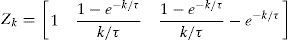
An alternative, suggested by Diebold and Li (2006), is to use some factors related to the estimation of the zero-coupon yield curve. This kind of model has been used for forecasting purposes given the good performance of the results. By determining beforehand the factors that characterize the shape of the term structure and use them in the X matrix it is possible to obtain better and more stable estimations. In fact, in a model with latent factors, such as that proposed by ABW (2008), the factors obtained are usually identified with some of the characteristics of the yield curve, like the level of interest rates or the slope (Litterman and Scheinkman, 1991; Chen and Scott, 1993). Along these lines, Diebold and Li (2006) proposal is to use the level (Lt), slope (St) and curvature (Ct) parameters from the Nelson and Siegel (1987) term structure specification as factors on an affine model. These factors can be found in most central bank estimations of the zero-coupon yield curve. This estimation imposes that nominal interest rates can be modeled4 as in Eq. (7).
In Eq. (7), τ, Lt, St and Ct are the parameters that give us the interest rate in time t with maturity in k periods. Diebold and Li (2006) propose fixing the value of τ in the mean value observed throughout the original sample,5 so interest rates can be considered affine to factors Lt, St and Ct. Therefore, values of these factors can be recovered as parameters in an OLS regression. Successive regressions in each period give us the time series of parameters Lt, St and Ct that can be considered as factors determining the term structure of interest rates. Lt, is the long-term interest rate (both forward and spot), St is the spread (difference between long-term and short-term interest), while Ct is a measure of the term structure curvature. Diebold and Li (2006) showed that all three parameters are needed in order to recover the whole structure of the yield curve.6 Restricting the parameters to just the level and the spread will entail the loss of the information about short-term changes in interest rates, usually linked to movements in inflation expectations.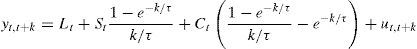
Nevertheless, Diebold and Li (2006) approach did not take into consideration the no arbitrage and risk aversion hypothesis, discarding Eqs. (4)–(6) of previous section. Moreover, as suggested by Carriero et al. (2006), including some macroeconomic variables in this framework could actually improve its performance.
In this paper we propose a model (we will refer as exogenous factors model) that simplifies the estimation procedure, and does not require any kind of ad-hoc restriction (like imposing an inflation price of risk equal to zero). Hence, we will define a model with four factors, three of them related to the shape of the yield curve, as proposed by Diebold and Li (2006), while the fourth (inflation rate) is included in order to subsequently be able to decompose the nominal interest rate. Additionally, we also impose no-arbitrage conditions following Annex 1, a suitable feature that was skipped by Diebold and Li (2006).
This solution goes in line with Kim and Orphanides (2005) proposal of including additional information in order to improve the estimations. Unfortunately, other kind of information apart of the parameters of the yield curve, such as survey forecast (Kim and Orphanides, 2005), or inflation-linked bond prices (D’Amico et al., 2007) are not always available.
Although including a fourth factor in the model may not be necessary in order to obtain a good fitting of the interest rate term structure if Nelson and Siegel model (Eq. (7)) is considered,7 adding the inflation rates allows us to taking into account that the yield curve provides information that could be useful in order to forecast inflation, what would have a clear effect on Eq. (2).
Since all factors in (8) are determined prior to the estimation of the affine model (Eqs. (1) and (2)), no restrictions, apart from (5) and (6) that ensure no-arbitrage and risk-aversion, are required on the model for the dynamics of Xt.8 Furthermore, there is no need of fixing any interest rate as observed without error, while initial values for the maximum likelihood estimation are easily obtained via OLS regressions (see Annex 2).
The closest model to the one here proposed is the one of ABW (2008) that includes both macro and latent factors in order to obtain a decomposition of US interest. The basic structure of the financial affine model with two latent factors is extended into a macro-finance affine model by adding the CPI rate as an observable variable to the VAR model.
Nevertheless, some restrictions have to be imposed to the parameters in order identify the estimation of the whole model.9 These restrictions are highly arbitrary as stated by Kim and Orphanides (2005). These authors also pointed out to the extra problems generally imposed in the estimation procedure with rather unstable results (especially for small samples and transition phases).
2.3Nominal interest rate decompositionOnce an affine model represented by Eqs. (1), (2) and (4) has been estimated, it is possible to decompose k-period nominal interest rates (yt,t+k) into real risk-free rates10(Ert,t+k), inflation expectations (Et[πt,t+k]) and risk premia11 (denoted by γt,t+k), according to Eq. (9).
Therefore, real risk-free rates (Ert,t+k) could be obtained by subtracting inflation expectations and risk premia from estimated nominal interest rates.
Firstly, inflation expectations are obtained from VAR Eq. (2). In fact, since vector Xt includes inflation (πt), expectations on this variable can be recovered from projections of the dynamics on the affine factors in the VAR Eq. (2).
Long-term nominal interest rate decomposition in Eq. (9) requires the average expected inflation for the aggregate period between t and t+k(Et[πt,t+k]), which could be recovered by integrating the forecasting values of inflation of Eq. (10) for consecutive periods between t and t+k(Et[πt+h,t+h+1]).
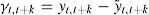
Secondly, risk premia are estimated as the difference between nominal interest rates and their risk-free counterpart. As stated in Section 3.1, the risk premium appears as a consequence of investors’ risk-aversion (see Annex 1). This factor only reflects the existence of uncertainty in the future value of the affine factors driven by perturbations ¿t of the VAR equation. If investors were indifferent to risk, no risk premium would be needed to compensate them for the uncertainty of holding assets with longer maturities instead of shorter ones. In such a framework, the recursive formulas of Annex 1.2 would be applied instead of those in Annex 1.1. This is equivalent to assuming that the price of risk is zero (λt=0) during the period considered (Ang and Piazzesi, 2003). Consequently, we can now define risk-free rates y˜t,t+k as the interest rates obtained from affine Eq. (11).
where parameters A˜k and B′˜k are equivalent to those of Eq. (1), but assuming null prices of risk (Annex 1.2). Differences between estimated nominal rates and estimated nominal risk-neutral rates will be the consequence of the introduction of risk-aversion and can be considered as risk compensation (risk premium).The risk premium (γt,t+k), defined by Eq. (12), will increase with the term considered as implied by the construction of the affine model (see Annex 1), and will be time-varying (governed by the price of risk of Eq. (4)).3An application to the Spanish economy3.1Interest rate developments in Spain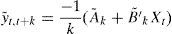
In order to better understand the results it would be useful first to provide an overview of the Spanish economic evolution during the 90s. During this period, the evolution of the nominal variables, like the interest rates, was closely related to the nominal convergence process associated with EMU entry, and by the structural and policy changes that were performed. In this sense, the economy moved from a scenario of high inflation rates and large public deficits to a new framework based on fiscal surpluses, moderate inflation and EMU membership. However, this was not a smooth process and was plagued by uncertainty related to the EMU process itself and the ability by the Spanish economy to fulfill the Maastricht convergence criteria. It seems likely that these uncertainties impinged on the expectations on several macroeconomic variables such as the inflation rate. In this sense the long run inflation expectations should have been a weighted average of the inflation rate under the convergence regime and the alternative inflation rate that could have prevailed under a non-convergence scenario. Under those circumstances, it seems obvious that the observed inflation rate is not a good proxy for inflation expectations nor is it a simple way of estimating those expectations.
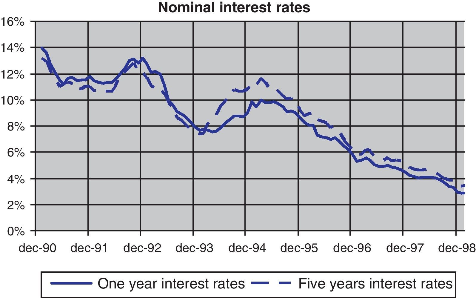
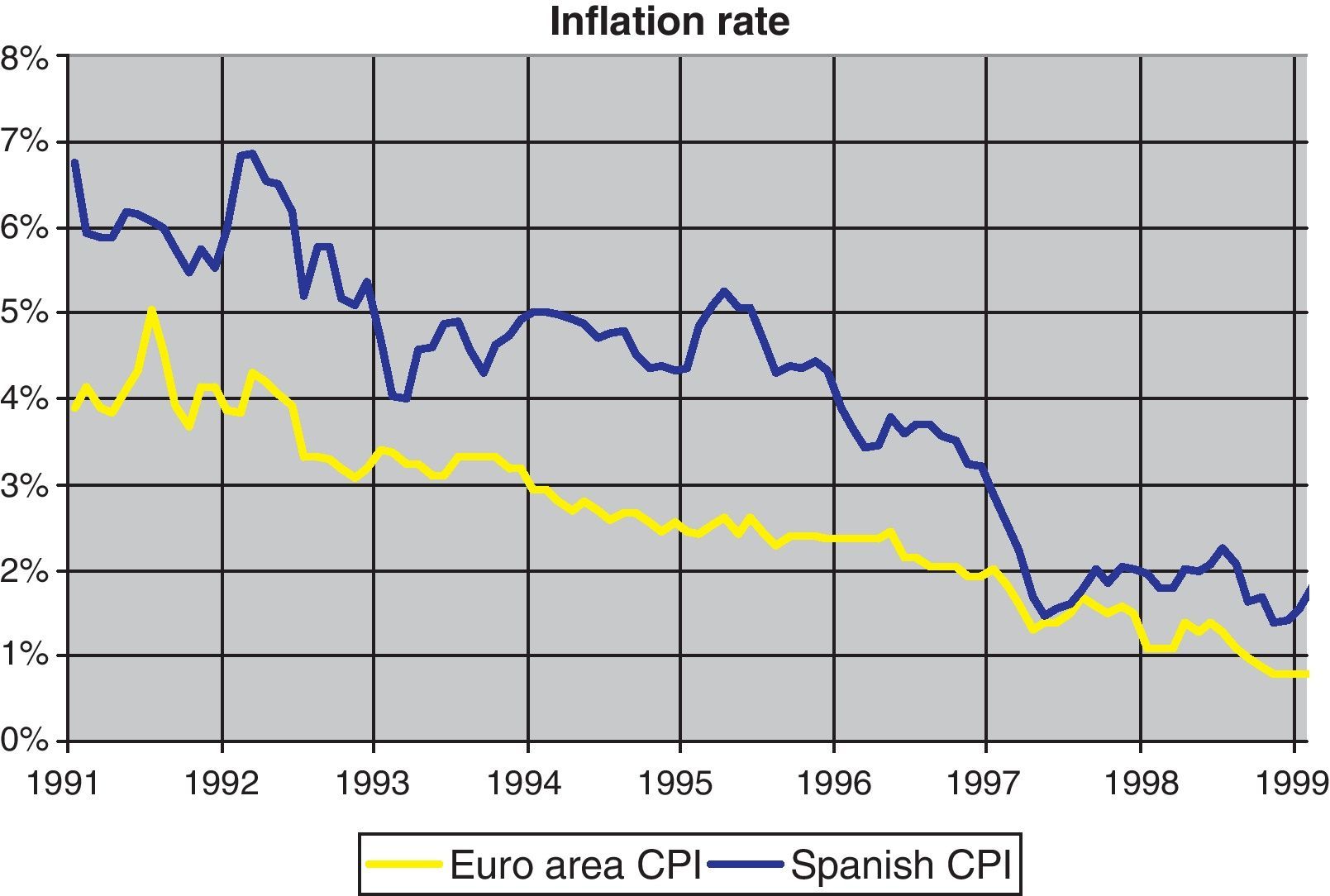
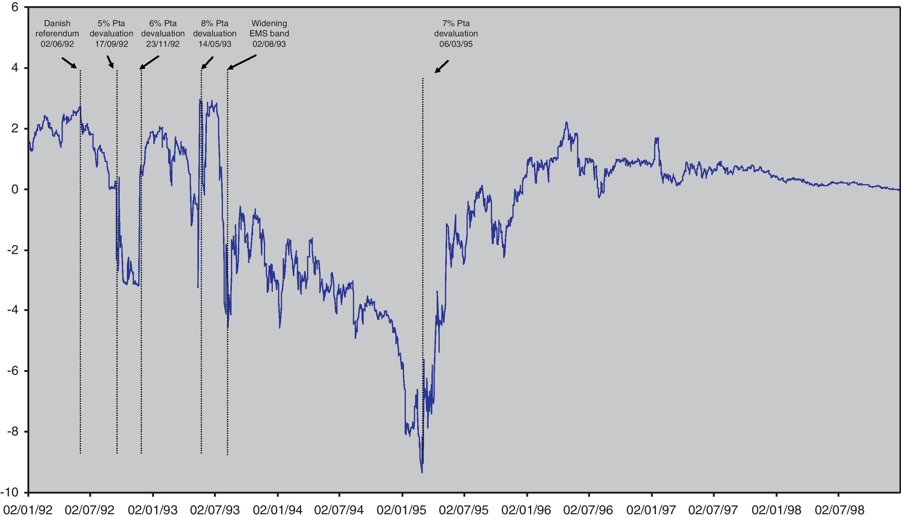
The financial markets also reflected these uncertainties. In fact, as can be seen in Fig. 1, Spanish nominal 5-years interest rate fell from 13–14% at the beginning of the decade to 3–4% at the end of the nineties reflecting a similar process than the inflation rate that can be seen in Fig. 2, where the Spanish inflation differential against the euro area narrowed from 3pp at the beginning of the decade to a value close to 1pp at the end of the nineties. Two peaks can be observed in the course of the reduction of nominal interest rates indicating the aforementioned uncertainty episodes: first, the European Monetary System crisis at the end of 1992; and second, the widening of the ERM bands in 1995. Moreover, the Peseta exchange rate was also affected by the uncertainty over the process. As Fig. 3 shows, the decade started with high variability of the Spanish Peseta exchange rate against the Deutsche Mark, which gave rise to four episodes of devaluation that coincide with the aforementioned peaks of 92–93 and 95.12


, depreciation (−) of nominal exchange rate of the Peseta against Deutsche mark central parity.")
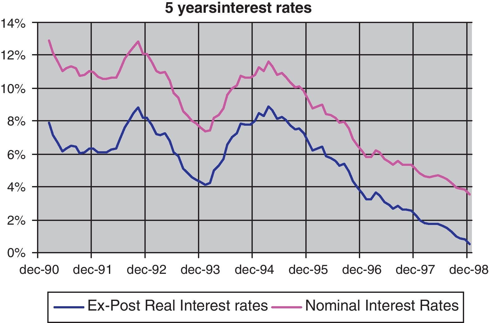
Under this framework, the ex-post real interest rates, which are normally used as a proxy for actual real interest rates, decreased significantly (see Fig. 4). However, the magnitude of this reduction (more than 6pp) seems to be excessive for it to be interpreted as a change in real risk-free interest rates.
3.2Data
In order to estimate the affine model proposed that we propose, we use monthly spot nominal interest rates for the Spanish Government Yield Curve.13 The interest rate time series considered in our analysis run from January 1991 to December 1998. The beginning of the sample is determined by the availability of data, while the end is given by entry into the European Monetary Union, and nominal interest rates began to be driven by European determinants. For the estimation of the parameters of the yield curve we use the interest rates from 1-month interest rates to 5-year interest rates, which give us 60 interest rates for each of the months considered.
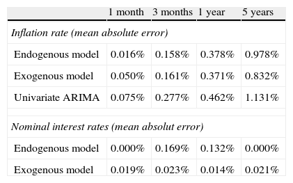
3.3Estimations resultsTable 1 shows the mean absolute error in both inflation rate forecasts and the interest rates fitting for our model and as for comparison purpose we also include the results with the alternative model of ABW based on endogenous factor. Additionally, as a benchmark, we include the projections for the inflation rate based on an ARIMA model that take into account only the lagged values of this variable and did not consider the market information contained on interest rates.
Mean absolute error in the estimated models.
| 1 month | 3 months | 1 year | 5 years | |
| Inflation rate (mean absolute error) | ||||
| Endogenous model | 0.016% | 0.158% | 0.378% | 0.978% |
| Exogenous model | 0.050% | 0.161% | 0.371% | 0.832% |
| Univariate ARIMA | 0.075% | 0.277% | 0.462% | 1.131% |
| Nominal interest rates (mean absolut error) | ||||
| Endogenous model | 0.000% | 0.169% | 0.132% | 0.000% |
| Exogenous model | 0.019% | 0.023% | 0.014% | 0.021% |
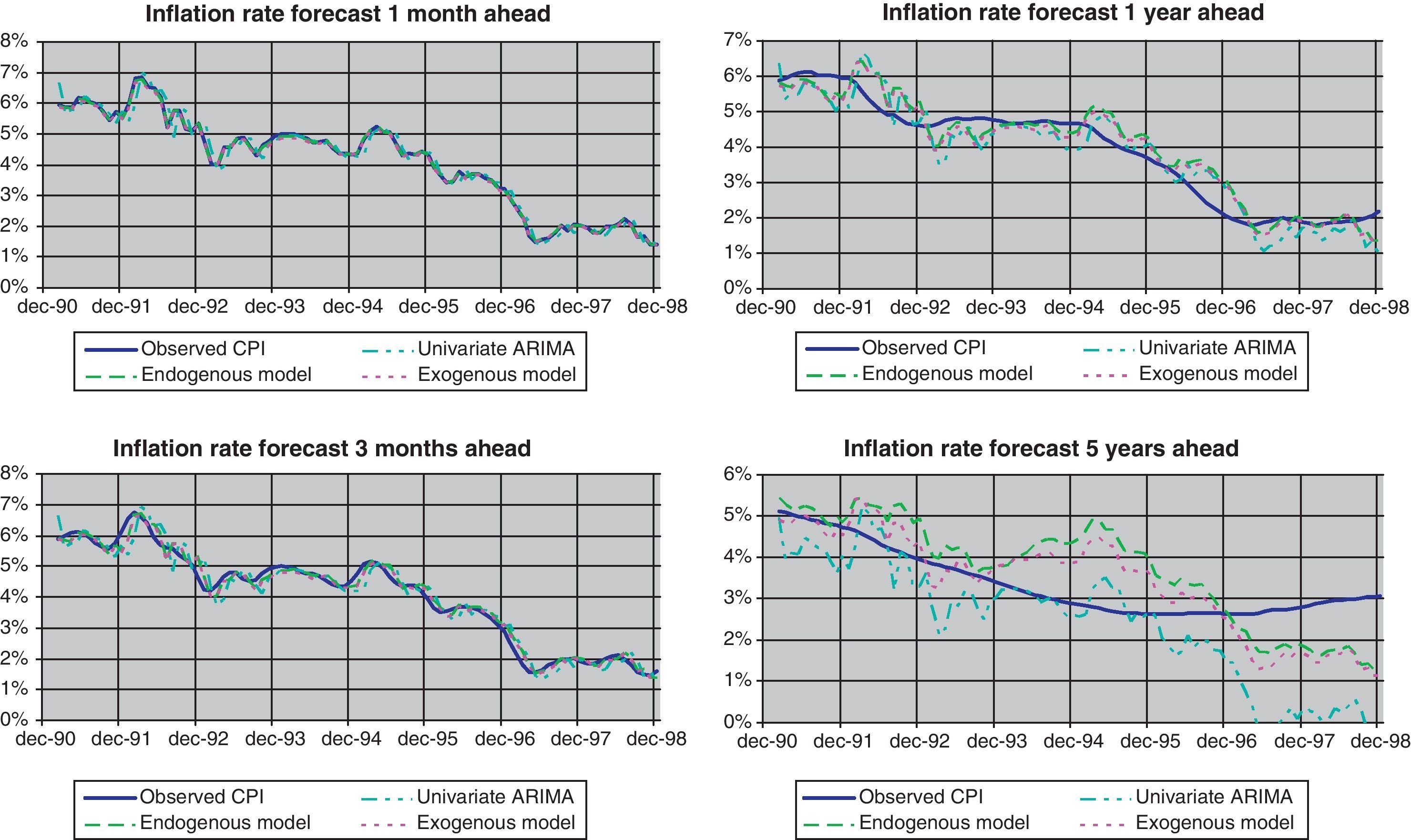
The goodness of fit differs depending on the equation considered. Affine models, irrespectively of the specification considered, capture the information contained in the term structure about the future course of inflation rate and outperform the projections from a univariate ARIMA. Nevertheless, no clear preference could be established between them, although longer horizon forecasts seem to be slightly better in the case of the exogenous model (see Fig. 5).

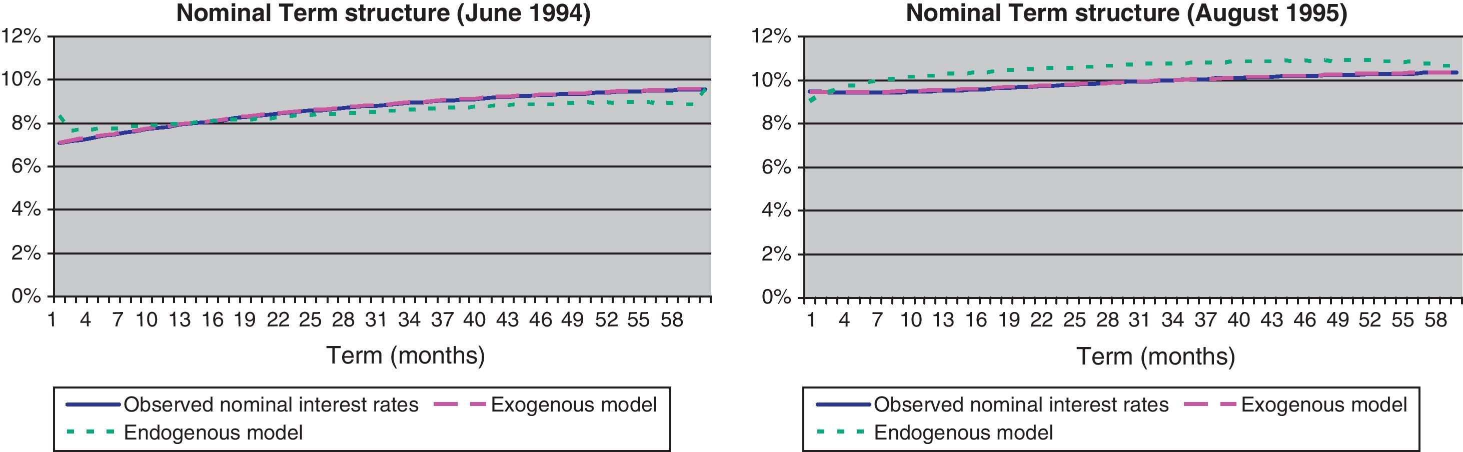
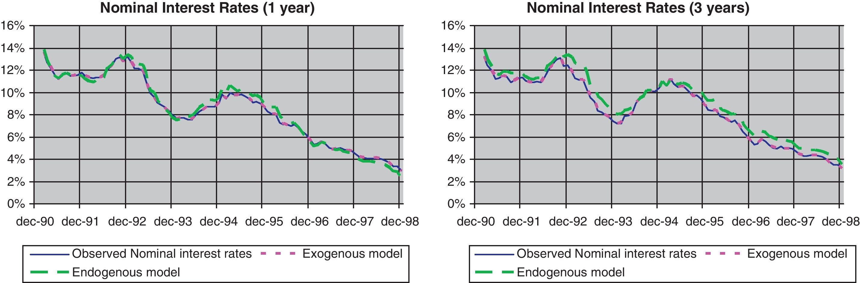
In the case of the term structure of the interest rates (Eq. (1)), results clearly show that our model outperformed the alternative based on endogenously determined factors. As can be seen in Table 1 and in Fig. 6, our estimation procedure produces better results in the 1 year and 5 years, that are the relevant terms for comparing the endogenous model, given that the estimation of the other terms has been required to be computed without error (3 months and 5 years in the output presented). This can be observed in Fig. 6 for two specific periods, in which the model with exogenous factors captures all the term structure, while the unobserved component allows for significant deviations along the yield curve. Fig. 7 also shows the better fitting of our model throughout the sample.

.")
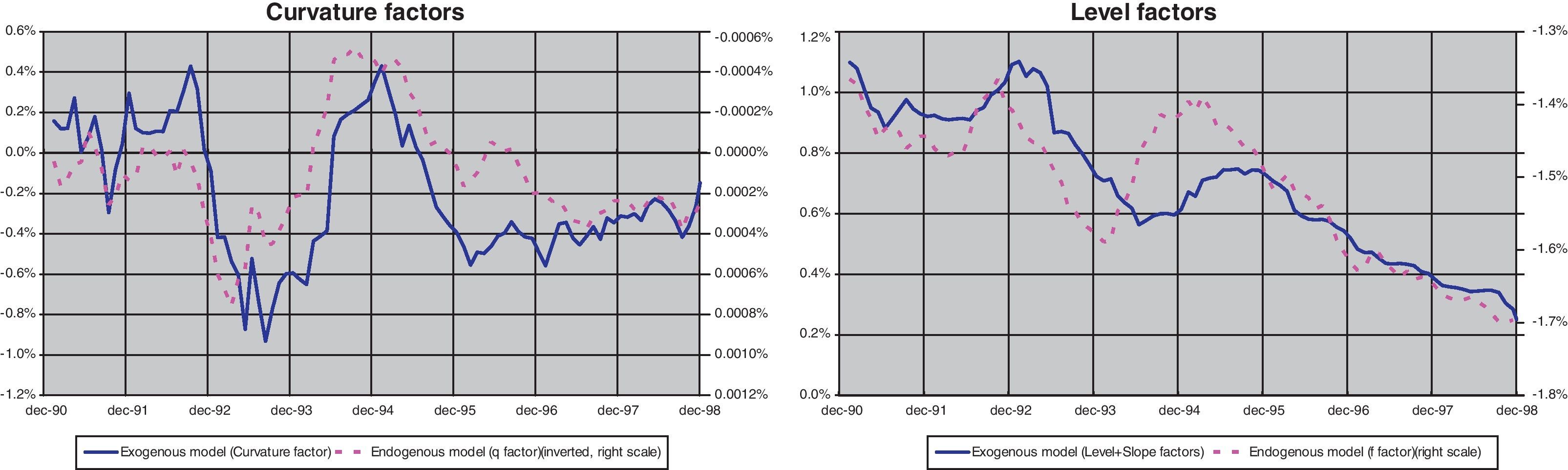
The problems of the performance of the endogenous model could be explained by several reasons. Firstly, we have to acknowledge that this model lacks one factor in comparison with the exogenous one. When compared, q factor has a close behavior to the one present in the curvature factor of the exogenous one (Fig. 8), while the f factor is similar to the addition of the long term level and slope factors (short term interest rates). By reducing one factor in the endogenous model, inflation expectations play the role of the difference between long-term and short-term interest rates, something that is not always the case.

Moreover, the number of parameters that has to be estimated along with the latent factors that have to be recovered usually gives rise to some problems of identification. In order to solve them, it is usual to impose some restrictions on the set of parameters. For instance, factors q and f are set to be independent while past values of inflation do not affect either of the latent factors. The main drawback of this approach is the reduction in the flexibility of the model, which could cause some difficulties in the accuracy of the estimated term structure.
In addition, the estimation procedure used by ABW (2008) requires assuming that a number of yields (equivalent to the number of latent variables) should be observed without error, in order to recover the unobserved latent factors. We have found that, at least in the Spanish nominal convergence process, the results are extremely sensitive to the interest rates selected as observed without error. We choose the 3-month to 5-year interest rates in order to take into account both extremes of the yield curve.
Finally, estimation results are extremely sensitive to the initial values of the parameters that have to be chosen arbitrarily. In order to avoid, to some extent, this problem, we have implemented a Genetic Algorithm (see Gimeno and Nave, 2009) excluding combinations of parameters that create meaningless estimations (such as consistently negative real interest rates or risk premia and extremely high values of inflation rates). This methodology, which is heavily demanding in computational terms, performs a better optimization by allowing the comparison of several sets of initial parameters.
By contrast, in our proposal the step-by-step estimation of Eqs. (1) and (2) (see Annex 2) is a good approach to the initial values in the joint maximum likelihood estimation for the whole model. Sensitivity to the initial values disappears, and Genetic Algorithms are not required either, reducing the computational time.
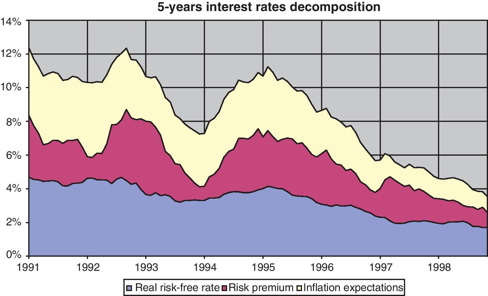
3.4DecompositionFrom Eq. (9) in the previous section, it is easy to see that once nominal interest rates have been stripped of both inflation expectations and risk premia, real risk-free rates will be the remaining value.14 This decomposition is represented in Fig. 9, where the course of the expected inflation in the next five years, and the risk premium associated with the uncertainty about term structure changes in this period are removed from five-year nominal interest rates.

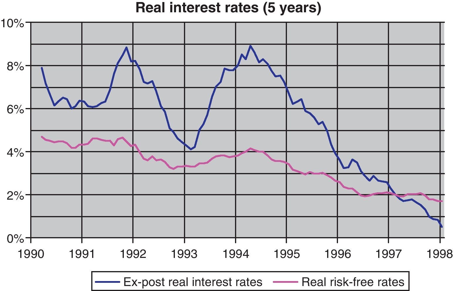
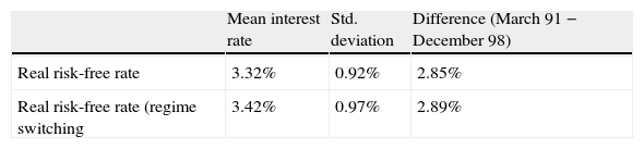
As can be seen, most of the decline in nominal interest rates came from the reduction in inflation expectations and a further decline in the risk premia, while real interest rates fell by less than 3pp during the sample period. The magnitude of this reduction in real risk-free interest rates is consistent with the findings of Blanco and Restoy (2011), in the sense that the evolution of macro and financial variables in the Spanish economy during this period did not support a reduction in the cost of capital similar to that suggested by ex-post real interest rates drop of 6.7pp (Fig. 10). Furthermore, results for real interest rates obtained with this model are in line with those obtained for other countries and methodologies (Laubach and Williams, 2003; Manrique and Marqués, 2004; Cuaresma et al., 2004 among others).

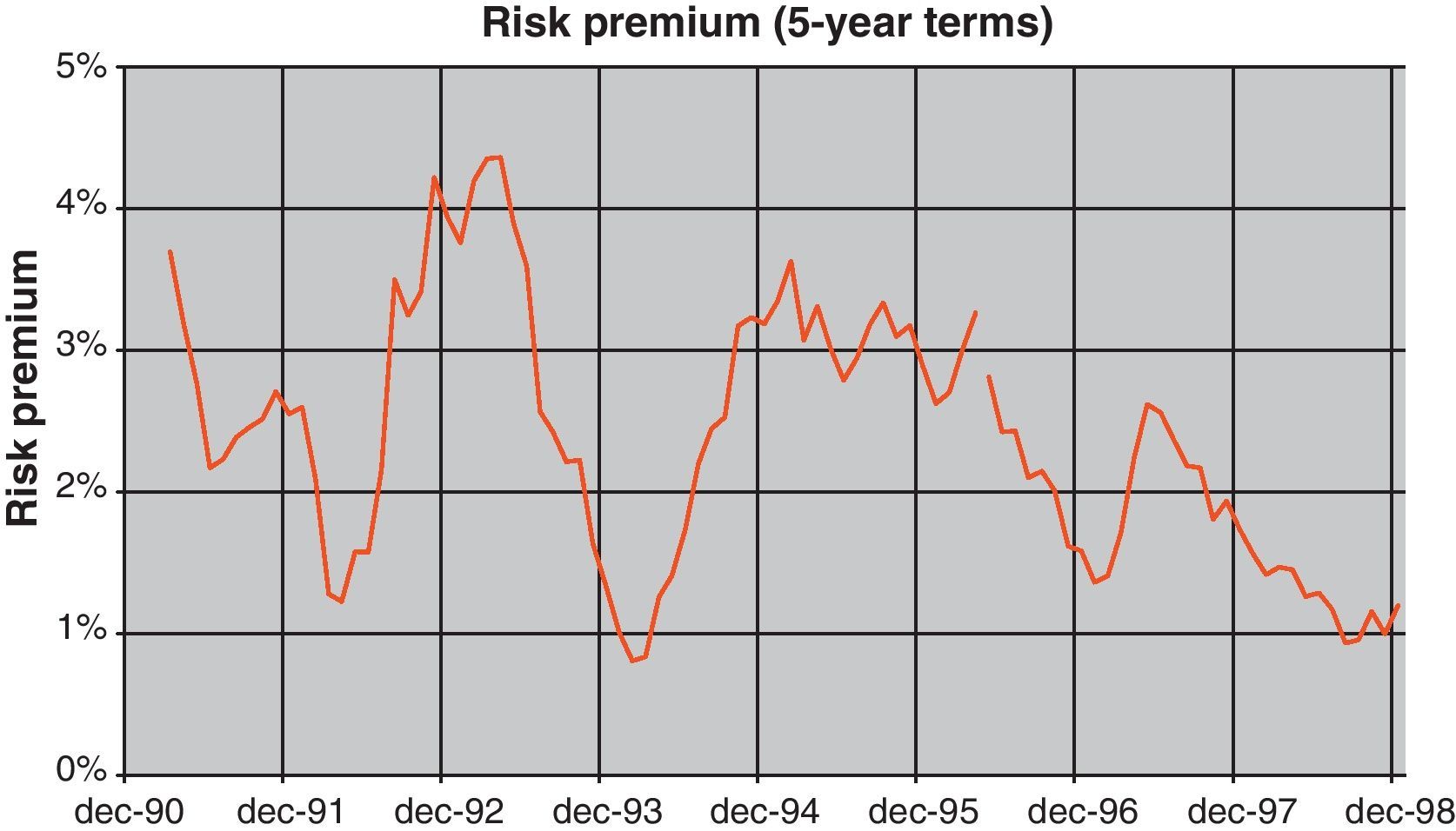
Most of the volatility in ex-post real interest rates is in fact captured by the estimated risk premium (see Fig. 11 for the estimated five-year risk premium). As can be seen, this magnitude had ample volatility in the period considered and, in fact, was responsible for a sizable share of nominal interest rate movements. In fact, the major increases in the risk premium occurred in periods of weaknesses of the Spanish currency and could be linked to market uncertainty about future interest rates and inflation in the event of devaluation. From the mid-nineties this uncertainty vanished due to the fact that it became increasingly clear that Spain would enter the euro area15 at the end of 1998.

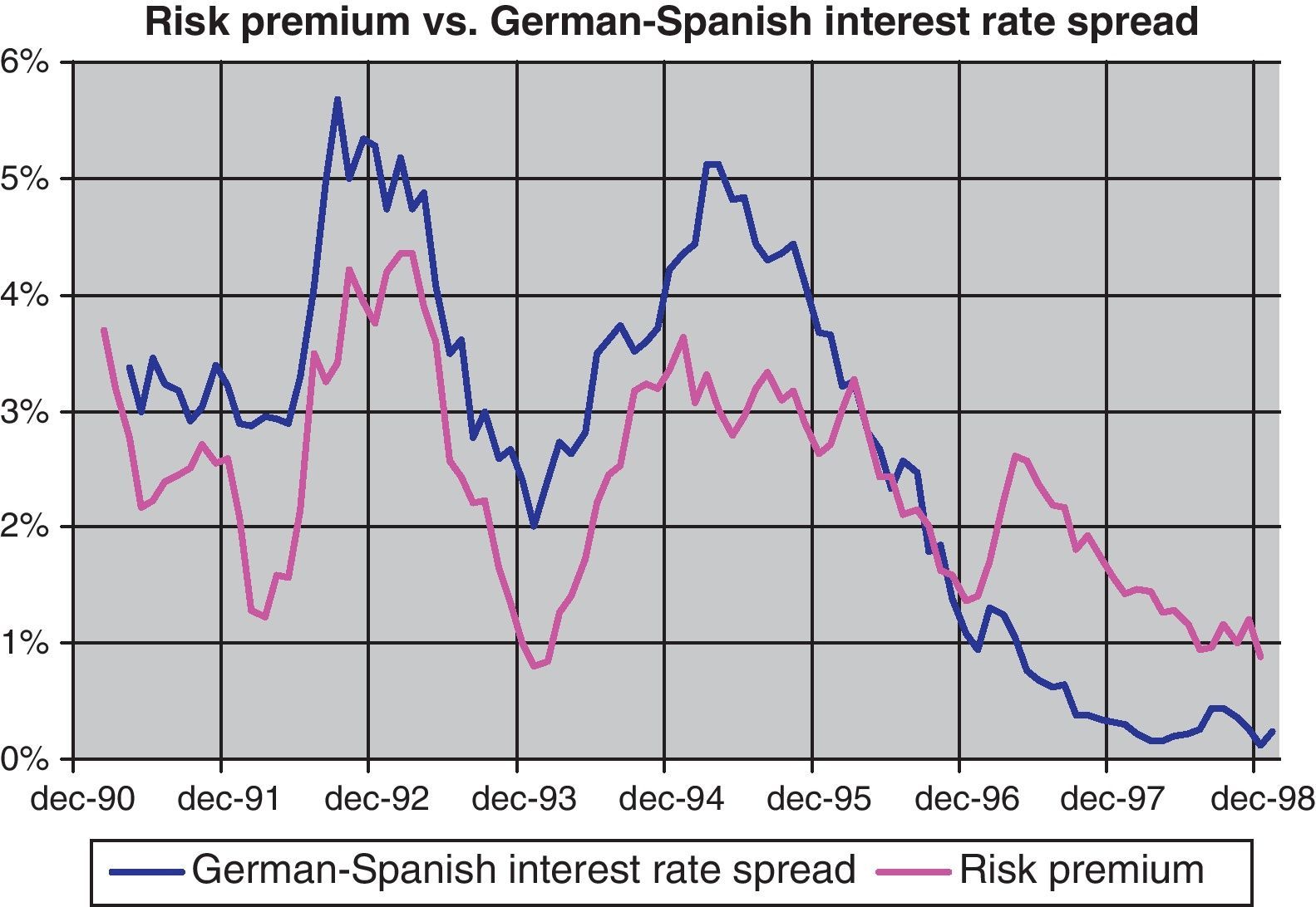
Indeed, if we compare (Fig. 12) the estimated risk premium with the spread between the Spanish bond yield and the benchmark German bund, we can see that not only does the magnitude of the risk premium matches the spread but also the evolution is strongly similar. This result is in line with the intuition that in a nominal convergence process towards a monetary union the changes in the spread should be closely linked to the probabilities assigned to the EMU entry. In fact, during this period some practitioners used the spread to extract the probabilities of entry into EMU (see Bates, 1999). It is easy to see that at the end of the decade both variables tend to diverge, signaling a switch in the link between the term structure and the Spanish CPI to the European index, once it was clear Spain was going to enter EMU.16

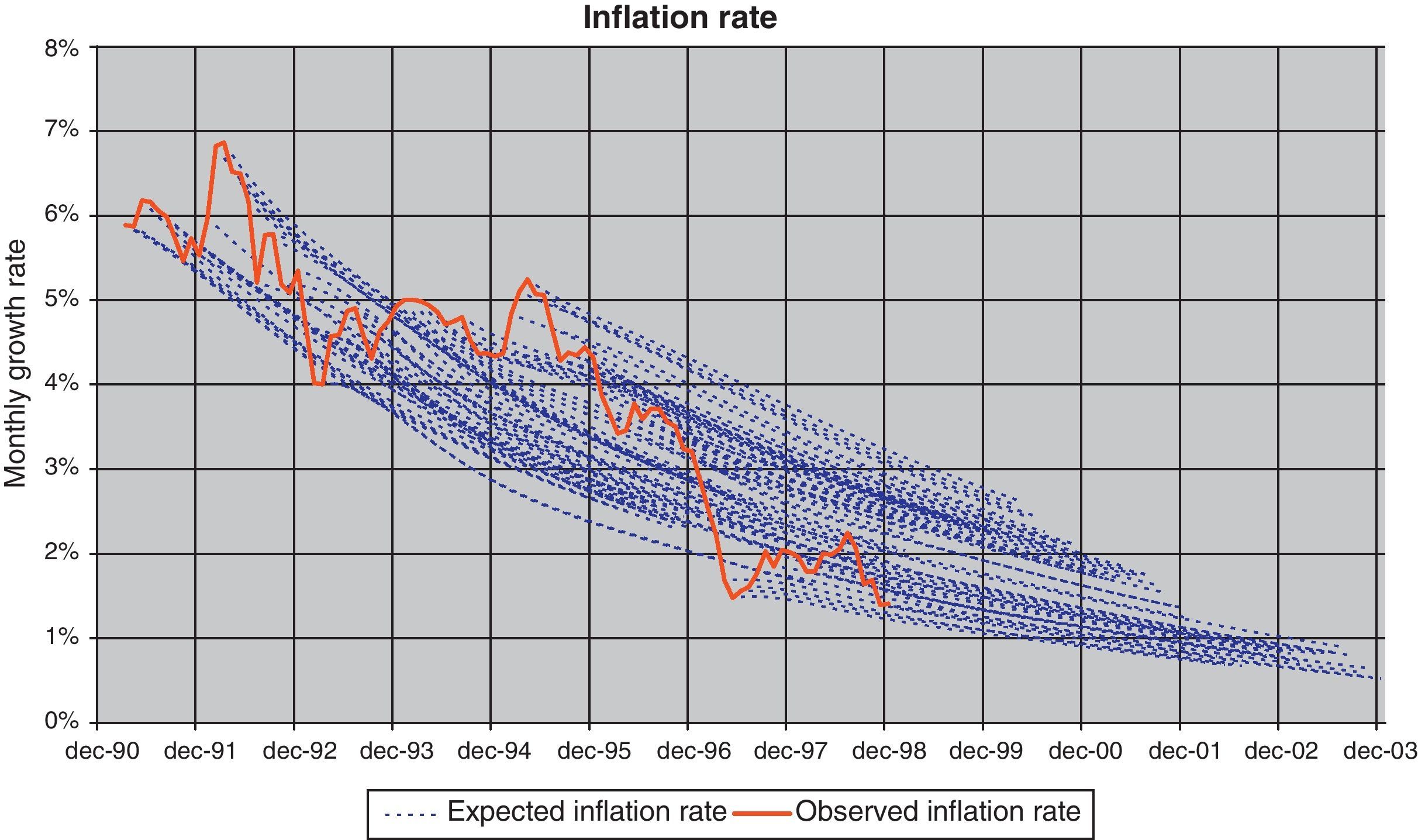
Finally, in the case of the CPI, projections obtained for different periods with Eq. (10) are presented in Fig. 13 (blue dotted lines) and compared against the observed CPI (unbroken red line). As can be seen, on average the paths of inflation projections are similar to those of observed inflation. Although the differences between projected and actual data increase with the prediction horizon, these differences are lower than those obtained via a univariate ARIMA (Table 1).

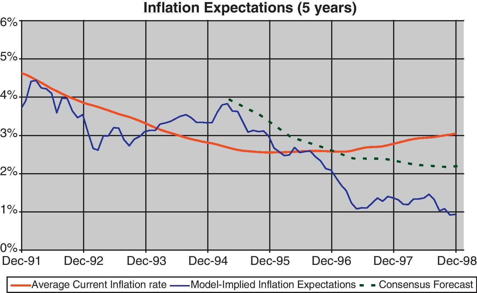
If we compare observed inflation and the CPI five-year forecast, following Eq. (10), as well as the evolution of the expectations derived from the Consensus Forecast, as shown in Fig. 14, we can find periods with both inflation expectations were persistently higher than the final actual values (i.e. 1994–1995), producing a divergence between ex-ante and ex-post interest rates. These differences were in line with some concern about Spain's entry into EMU that would have affected inflation expectations as well as the associated risk premium, and would have been reflected in the evolution of the term structure. However, in the final year of the sample, where there was a general consensus about the entrance in the EMU, both types of inflation forecasts (survey and estimates) produced outcomes lower than the finally observed. The reason could be related with some expectations of convergence between the Spanish and the euro-area inflation rate that was not finally achieved after entering to the euro-zone. In fact, in the following years a persistent inflation gap was observed between Spain and the euro-zone. This evolution, which could be not anticipated by most of the analyst, could be due to the fact that the process of wage and price formation continued to be referred to national references instead to the euro area benchmark (see Alberola and Marqués, 2001).

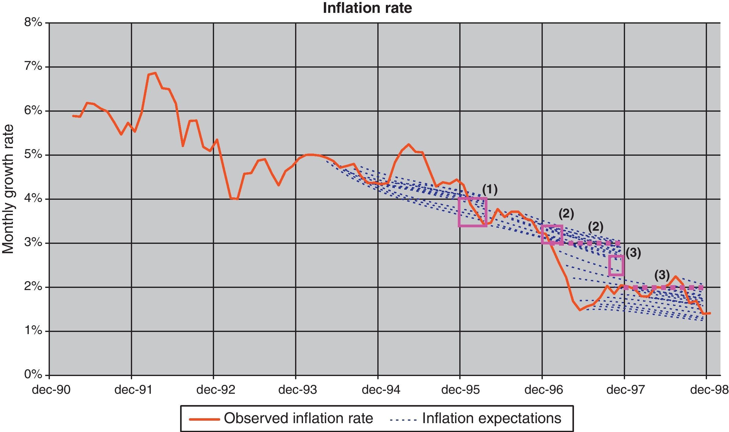
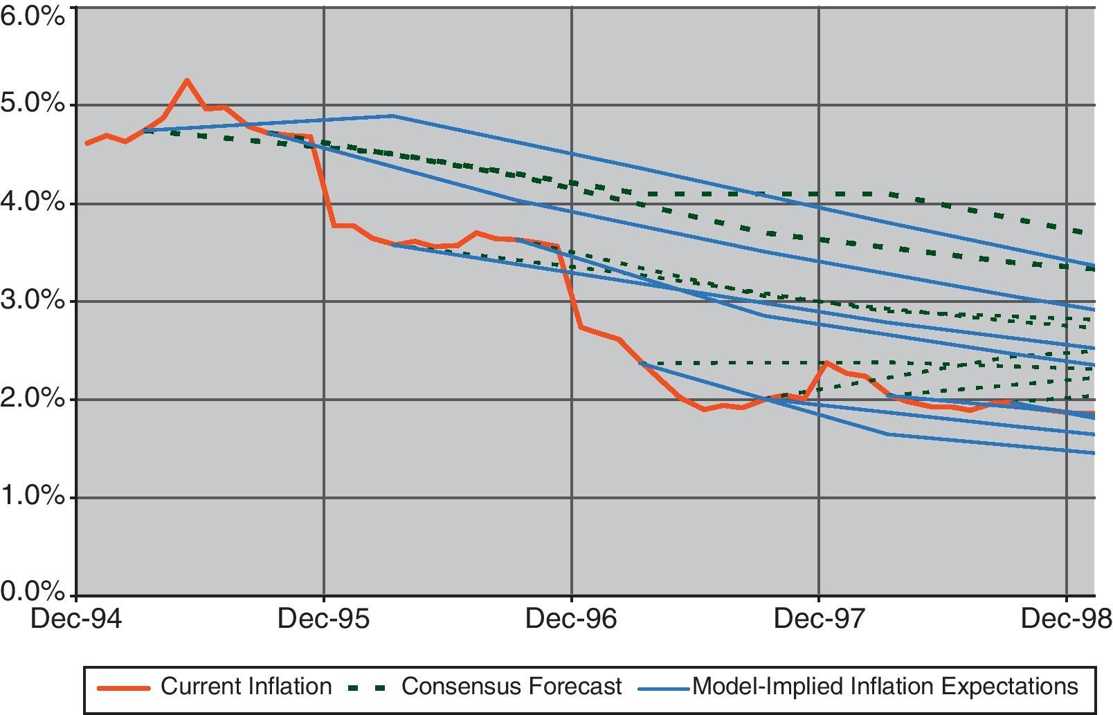
In fact, the information content in the fixed-income markets about the CPI via the term structure found with this model highlights the credibility given by the market to the inflation targets published by the Banco de España during that period in its inflation report. In Fig. 15 the inflation targets set by the Banco de España (represented by the red square and the dotted red lines) are compared with the market projections implied by the term structure and obtained with Eq. (10), showing a close relationship between them. Same result is observed when inflation expectations are compared with the consensus forecast (Fig. 16). In fact, this feature, reinforce the evidence of the term structure information contents on inflation expectations.
 CPI target: between 3.5% and 4% at the beginning of 1996 (p. 13, Economic Bulletin, December 94, Banco de España). (2) CPI target: close to 3% at the beginning of 1997 and below it during the year (p. 12, Economic Bulletin, December 95, Banco de España). (3) CPI target: around 2.5% at the end of 1997 and close to 2% in 1998 (p. 12, Economic Bulletin, December 96, Banco de España).")
Banco de España inflation targets and model projections.
(1) CPI target: between 3.5% and 4% at the beginning of 1996 (p. 13, Economic Bulletin, December 94, Banco de España).
(2) CPI target: close to 3% at the beginning of 1997 and below it during the year (p. 12, Economic Bulletin, December 95, Banco de España).
(3) CPI target: around 2.5% at the end of 1997 and close to 2% in 1998 (p. 12, Economic Bulletin, December 96, Banco de España).

Some studies, such as ABW (2008), include a regime switch in their model affecting both the level of affine variables (the drift in Eq. (2)) and the risk premium (via the Σ matrix, or the price of risk equation). In this sense, ABW (2008) consider two regimes in order to take into account differences in monetary policy strategy and different cyclical positions. The same approach could be of interest in the Spanish case as a possible means of capturing the nominal convergence process that ended upon EMU entry.
In order to implement a Markov regime switch in our exogenous model we consider two different states (st) which, in theory, could be linked to the convergence or not towards EMU. These two regimes would be associated with two states for the drifts μ(st) in Eq. (2) allowing for different inflation expectations depending on the state, as well as two different vectors of constants λ0(st) for the price of risk in Eq. (4) to account for different uncertainty valuation.

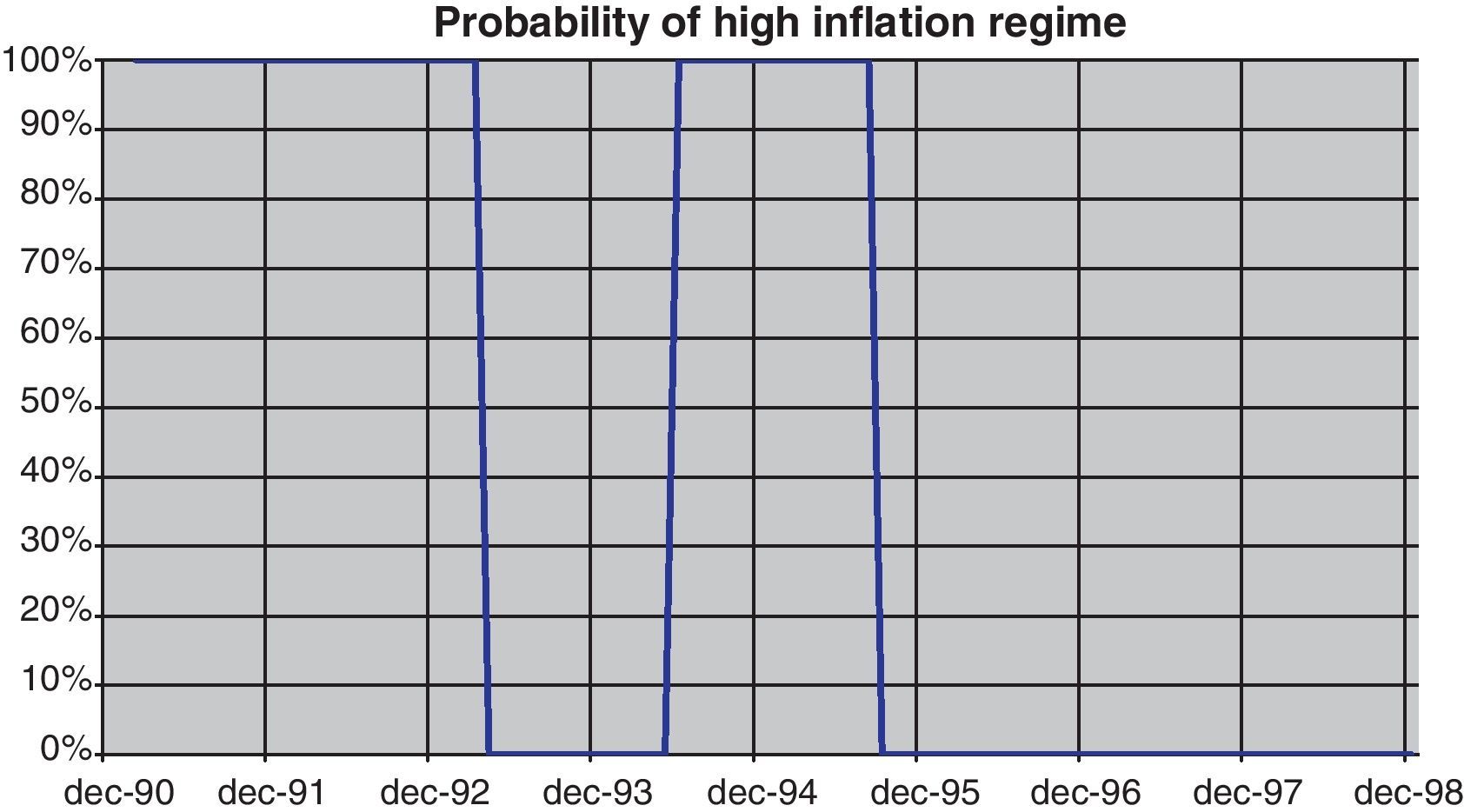
Two regimes, one of them of low inflation, are therefore identified. As can be seen in Fig. 17, the regime of high inflation appears to be most likely at the beginning of the nineties and around 1995. Both episodes were characterized by currency turbulence and serious market doubts about Spanish fulfillment of the Maastricht criteria and EMU entry.

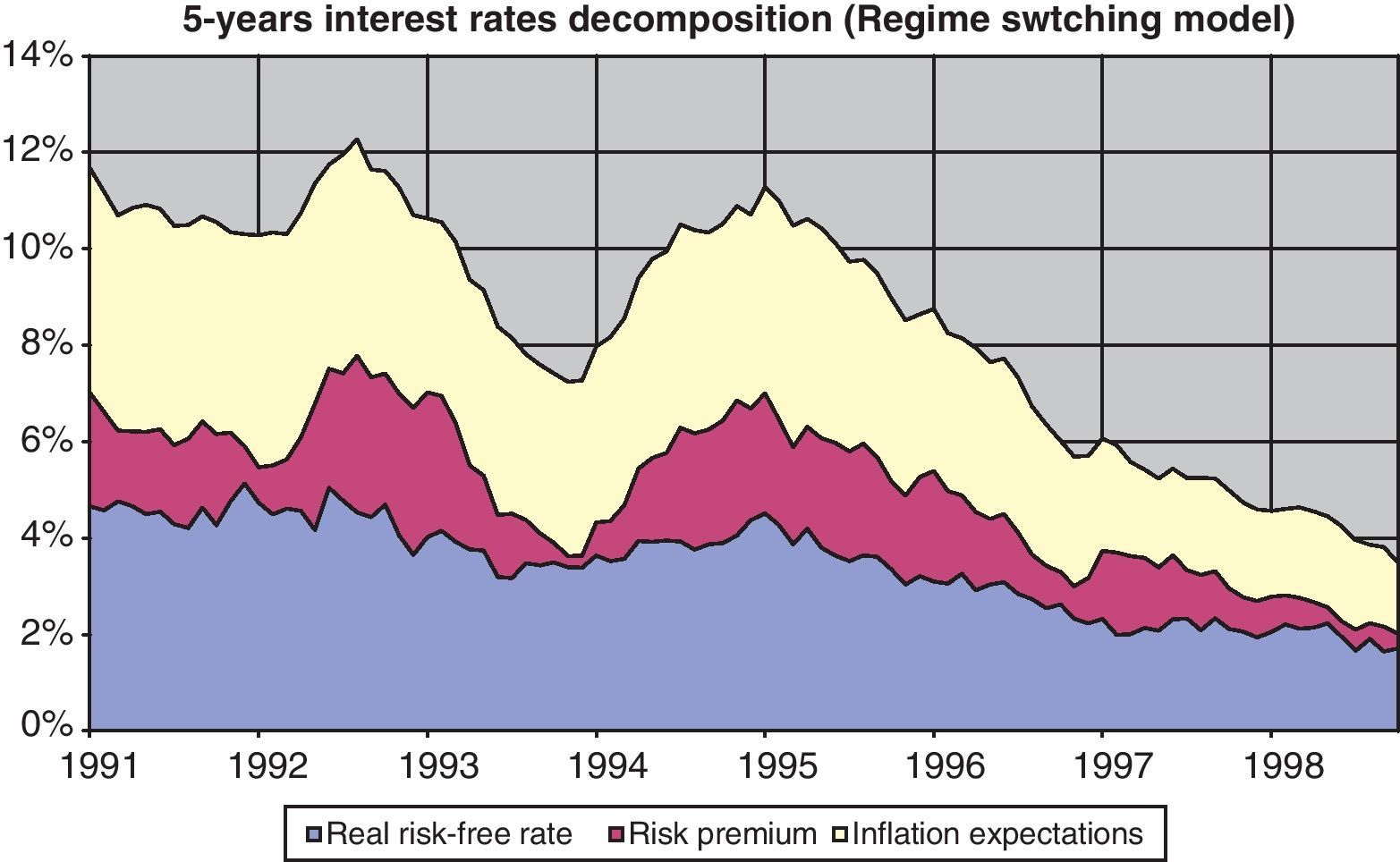
The results of the (exogenous17) regime switching model are highlighted in Fig. 18, which evidences the nominal interest rate decomposition, similar to that presented in the previous section for the model with just one regime. Slight differences between both models are reflected in a swap between inflation expectations and risk premia. The appearance of a second state of higher inflation increases both the overall expectations as well as the compensation given in nominal interest rates. But this increase implies that CPI expectations reflect the possibility of a higher inflation regime, reducing the upside risk and increasing the downside one, so this rise is balanced by a reduction of the same intensity in the risk premium.

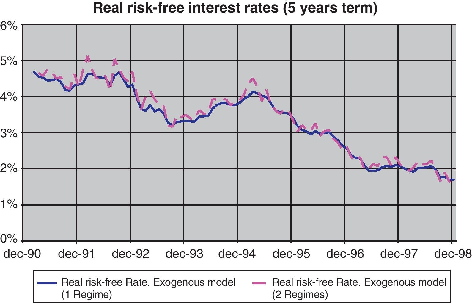
In this respect, as shown by Fig. 19, real risk-free rates seem to be not affected by the introduction of a regime switch, giving both estimations a very similar path for real risk-free rates. In fact, the intensity of the fall in interest rates is independent of the use or not of the Markov regime switch (Table 2) and the transition in real risk-free rates produced by the convergence process of the nineties can be fully explained by our model without any need of adding regime switching.
4Conclusions. 1 regime vs. 2 regimes.")
In this paper we discuss the decomposition of nominal interest rates for Spain under an affine model methodology that only imposes risk-aversion and no-arbitrage opportunities along the yield curve. We propose the use of exogenously determined factors based on the zero coupon yield curve estimation and compare the results with standard endogenously determined factors. Our results suggest that exogenously determined factors related to the estimation of the zero coupon curve exhibit the best properties in term of robustness, fitness and economic interpretation of the results.
Therefore, this kind of exogenously determined factors seems to be more appropriate for obtaining the decomposition of interest rates. These results could be of special interest in the case of a country involved in a nominal convergence process (like the accession countries to the European Monetary Union) or with changes in the monetary policy strategy implemented by the central bank (like the Federal Reserve during the Volcker period). The Spanish economy during the 90s, a period previous to the entry in the European Monetary Union, supposes a good example of both situations.
Interest rate decomposition obtained for Spain points to a real risk-free interest rate reduction of less than 3pp during the nineties, a figure substantially lower than the ex-post real interest rate reduction and the decline previously found in the literature with other methodologies. This magnitude seems to be close to that observed in other countries and reflects the fact that most of the reduction in nominal interest rates during that decade can be attributed to a decline in risk premia and the convergence of inflation expectations towards European values.
A no-arbitrage condition guarantees the existence of a risk-neutral measure (noted as Q) that allows interest rates to be expressed in terms of future term structure outcomes,

Risk-neutral measures (Q) are usually converted into natural probabilities using the Radon–Nikodym derivative, as in Ang and Piazzesi (2003), denoted by ξt,
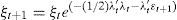
Usually, ξt in Eq. (A.2) is assumed to follow a log-normal process,where λt is a time-varying vector that incorporates the concept of risk-aversion into the valuation framework. The first part of the exponent (λ′tλt) is the Jensen Convexity component that ensures that Et[ξt+1/ξt]=1, while in the second, λt multiplies the perturbation vector εt+1, scaling the uncertainty in the random variables. This second term is responsible for the introduction of the risk premium in the valuation framework, whereby λt can be considered as a price of risk. Time-variant risk premia (Bekaert and Hodrick, 2001) will be the consequence of changes in this price of risk that is modeled assuming it to be also affine to the same factors Xt,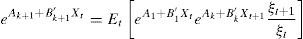

Finally, substituting (A.3) in (A.2), we arrive at a modified no-arbitrage condition that now takes into account investors’ risk aversion.
Only Xt+1 and εt+1 of expression (A.5) are not already known in period t, while the other terms in the exponents can be extracted from the expectations operator,

Nevertheless, vector Xt+1 can be forecast using VAR Eq. (2),
The exponent left in the expectations operator of expression (A.7) is solved taking into account the Jensen inequality.Finally, replacing the price of risk λt in (A.8) by its definition (Eq. (A.4)), we arrive at expression (A.9),This last expression allows us to recover the recursive expression of coefficients Ak+1 and B′k+1 in the affine representation as a function of the shorter terms,


The risk neutrality valuation framework used in (A.1) allowed us to incorporate the risk premium into the term structure. In order to recover risk-free rates we should consider a framework where agents are not concern about risk, so expectations derived from the non-arbitrage condition are evaluated under a natural measure,
where A˜j and B˜′j are the coefficients of Eq. (1), that meet no-arbitrage conditions. Using the same reasoning of Annex 1.1, replacing Xt+1 by its forecast and applying Jensen inequality to solve the expectations operator we arrive at expression (B.2),As can be seen, expression (B.2) is equivalent to (A.8), the only difference being that once you avoid risk-aversion the term B′kΣλt is no longer needed. In fact, this was the term that added a risk premium for each extra period of investment. A risk-neutral individual would have a null price of risk, with both expressions becoming equivalent. Under this assumption, the term structure recursive expression would be now,

Prior to the estimation of the affine model we have to determine the factors related to the term structure. Following Diebold and Li (2006), we use the Nelson and Siegel (1987) formula of the term structure.
Diebold and Li (2006) fixed the value of τ to be the mean throughout the sample. Once τ is constant, Eq. (C.1) can be estimated by OLS for each period, regressing interest rates for different terms (k) against matrix Zt.
Once Lt, St and Ct are estimated as the parameters of these regressions for each period, they can be used as factors for the affine model. As vector Xt is completely determined, we no longer need to fix any interest rate as observed without error. In fact, it is now quite easy to recover initial values of the parameters via OLS estimations in three steps.
Since vector Xt is exogenously determined, we can estimate the VAR equation via OLS, which allows initial values to be obtained of μ, Φ and ∑

We can also use vector Xt to regress it against nominal interest rates for different terms using the term structure equation, in order to estimate consecutive values of Ak and B′k,

Finally, in order to incorporating non-arbitrage condition and risk aversion we go further than Diebold and Li (2006) and use Aˆk and B′ˆk estimations to regress them against shorter terms values, rearranging Eqs. (5) and (6). Once we have tentative values from (C.3) and (C.3), then Eqs. (5) and (6) become,
Eqs. (C.5) and (C.6) are linear with respect to λ0 and λ1, and therefore, these parameters can also be estimated by OLS.

Once we have estimated separately (C.3), (C.4), (C.5) and (C.6) equations, we have tentative initial values of the affine model that allow for a fast computation of the joint maximum likelihood estimation of the affine model given by,
We thank J. Ayuso, R. Blanco, Albert Lee Chun, Fernando Restoy, Itzhak Venezia the participants at the seminars at the Banco de España, the Business School of the Hebrew University and the HEC of Montreal for their useful comments. We are also thankful to the Sanger Chair of Banking and Risk Management of the HUJ for its financial support, and the project grant ECO2009-13616/ECON of Ministerio de Ciencia y Teconología.

