


The analysis of the structural behaviour of heterogeneous materials is a topic of research in the engineering field. Some heterogeneous materials have a macro-scale behaviour that cannot be predicted without considering the complex processes that occur in lower dimensional scales. Therefore, multi-scale approaches are often proposed in the literature to better predict the homogeneous mechanical properties of these materials. This work uses a multi-scale numerical transition technique, suitable for simulating heterogeneous materials, and combines it with a meshless method – the Radial Point Interpolation Method (RPIM) [1]. Meshless methods only require an unstructured nodal distribution to discretize the problem domain. In the case of the RPIM, the numerical integration of the integro-differential equation from the Galerkin weak form is performed using a background integration mesh. The nodal connectivity is enforced by the overlap of influence-domains defined in each integration point. In this work, using a plane-strain formulation, representative volume elements (RVE) are modelled and periodic boundary conditions are imposed on them. A computational homogenization is implemented and effective elastic properties of a composite material are determined. In the end, the solutions obtained using the RPIM and also a lower-order Finite Element Method are compared with the ones provided in literature.
Composite structures have been used in the engineering field in the past few decades and settled as materials for primary structural components in industries such as aircraft, aerospace or automotive. Their high specific mechanical properties and low weight make them ideal solutions for these applications. Thus, their structural analysis needs to be accurate and efficient.
The analysis of a composite material can be performed according to two different approaches that are often coupled in numerical frameworks: the macromechanical analysis and the micromechanical analysis. In macromechanics, the composite structure is considered as an homogeneous orthotropic continuum [2]. In this case, it is not considered the micro-heterogeneity of the composite material, which is a sufficient consideration for the majority of the engineering applications. Nevertheless, for more complex situations (such as micro-cracking or buckling of fibres), where the microscopic phenomena considerably influences the behaviour of the material at the macroscale, the micromechanical analysis is a more appropriate approach [3]. Thus, distinct multi-scale approaches are often found in the literature considering coupled analysis at different scales.
This work proposes a new micromechanical computational tool capable of being applied to a wide range of heterogeneous materials. This research is based on existing multi-scale numerical transition techniques [3–9] suitable for simulating heterogeneous materials assuming different arrangements of fibres in a fibre composite material and Representative Volume Elements (RVE) statistically representing the microstructure of the material and containing the information of the elastic constants and fibre volume fraction of the composite material. Using the scale transition theory, a homogenization procedure can be implemented at each infinitesimal point of the macro-scale (represented by the RVE), and homogenized elastic properties can be determined. These micromechanical principals are implemented within the formulation of an advanced discretization technique – the Radial Point Interpolation Method – and also a lower order Finite Element Method (FEM).
2Meshless methodsIn meshless methods, the problem domain is discretized in a set of nodes which are intrinsically independent from each other. Unlike the FEM, in meshless methods the field variables are approximated within an ‘influence-domain’ rather than an element [1]. It is also the overlap of influence-domains that ensures the nodal connectivity in these methods. ‘Influence-domains’ are areas or volumes (if the considered problem is bidimensional or tridimensional, respectively) concentric with an interest point [1], containing a certain number of nodes. The high nodal connectivity, and the fact that they are not mesh reliant, makes meshless methods advanced discretization techniques that are solid alternatives to the FEM.
As regards the integration mesh, it be can nodal dependent or independent, being the last case called a ‘not-truly’ meshless method since the mesh-free characteristic of these methods is not verified in that case (the method requires a background integration mesh). In comparison to the FEM, in meshless methods the shape functions have virtually a higher order, allowing a higher continuity and reproducibility [1]. Additionally, meshless methods can easily handle situations where the geometry is transitory such as problems involving large deformations or fracture mechanics – which are frequently associated, in the FEM, with re-meshing procedures showing high computational costs.
Another advantage of meshless methods concerns the simplified refinement procedure of the nodal mesh, which can be easily changed (by adding or removing nodes) [10]. Also, the solutions obtained from the meshless methods can be more accurate when compared with a lower order FEM [10], as will be shown in this study.
The first proposed meshless method was the Smooth Particle Hydrodynamics Method (SPH) [11] in 1977, but the first global weak form based meshless method was only presented in 1994 with the Element Free Galerkin Method (EFGM) [12]. From that date, other meshless methods were presented in literature such as the Meshless Local Petrov–Galerkin Method (MLPG) [13], the Reproducing Kernel Particle Method (RKPM) [14], Point Interpolation Method (PIM) [15], the Point Assembly Method [16], the Radial Point Interpolation Method (RPIM) [17] or the Natural Neighbour Radial Point Interpolation Method (NNRPIM) [1,18]. These meshless methods have been used in the past decades in several engineering applications and prove to be reliable and accurate numerical tools.
In the past years, some of the mentioned meshless methods were used in the field of computational homogenization and multi-scale approaches. For instance, the RPIM was used to impose periodic boundary conditions for the representative volume element (RVE) model of a 3D braided composite by Wang et al. [19]. The determination of homogenized elastic properties was a topic of interest of Falzon and Muthu [20] when using the EFGM for constructing an RVE. Wang and Liew [21] used a meshless method based on the moving least-squares (MLS) approximation and the EFGM for a micromechanical study of carbon nanotubes; Ahmadi et al. [22] used a truly meshless method based on the integral form of energy equation to study the steady-state heat conduction in an RVE of anisotropic and heterogeneous materials. Ahmadi and Aghdam [22], using the same meshless method previously mentioned, studied micro-stresses in a unidirectional fibre reinforced composite material which is subjected to a normal and a shear load; Rastkar et al. used an asymptotic homogenization and a meshfree Solution Structure Method (SSM) to obtain homogenized material properties; Yang et al. [23] presented a multiscale method for crack propagation using a Meshfree Adaptive Multiscale Method for Fracture (MAMMF).
In this work, the RPIM formulation is used for the micromechanical analysis of composite materials using RVEs defined in a plane-strain state.
2.1The Radial Point Interpolation MethodThe RPIM was created from the Point Interpolation Method (PIM) [15]. Using the polynomial basis function (as the PIM) and also introducing an additional radial basis function (RBF), the interpolation functions of the RPIM become more stable and robust than the ones used in the PIM.
This meshless method has been used in inelastic analysis of 2D solids [24], 3D contact problems [25], crack growth modelling in elastic solids [26], non-local constitutive damage models or even the bending [10,27] and dynamic [28–30] analysis of composite plates and shells. In this study, the RPIM will be used for micromechanical analyses of composite materials.
In the following subsections, the formulation of the RPIM is presented.
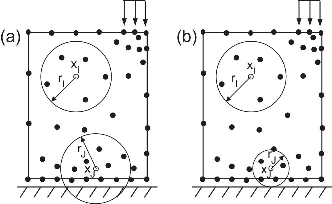
2.1.1Influence-domain concept. Nodal connectivityAs it was stated before, the nodal connectivity in the RPIM is imposed by an overlap rule between ‘influence-domains’, created following the nodal discretization (which can be regular or irregular, with the last case having, in general, lower accuracy) and the position of the integration point from the integration mesh. The influence-domain can have a fixed size (containing a well-defined number of nodes closer to a certain interest point) or a variable size, which consists in creating circles or rectangles concentric with an interest point and the nodes placed within those areas belong to the influence-domain of that interest point – Fig. 1. The literature recommends [1] the use of ‘influence-domains’ with the same number of nodes inside (for 2D problems, it is recommended between 9 and 16 nodes per ‘influence-domain’ [17]), which allows the construction of shape functions with the same degree of complexity.
2.1.2Numerical integration Variable size influence-domain (rI=rJ but the number of nodes within each influence-domain is different); (b) Fixed size influence-domain (rI≠rJ but the number of nodes within each influence-domain is the same).")
In the RPIM, the differential equations of the Galerkin weak form are integrated using background integration mesh composed by quadrilateral cells (using isoparametric quadrilateral shape) and in each cell are placed the Gauss integration points. The integration mesh can be fitted to the problem domain or can have a regular shape (in this case, the integration points placed outside the problem domain need to be removed). This numerical integration approach for solving the discrete system of equations does not meet the designation of a “truly” meshless method since the background integration mesh is independent from the nodal distribution. Indeed, the numerical integration performed in the RPIM is similar to the procedure followed in the FEM.
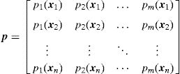
2.2Interpolation functionsIn the RPIM, the interpolation functions are obtained through the combination of polynomial basis functions with multi-quadric radial basis functions (proposed initially by Hardy [31]). Consider the influence-domain Ω of the interest point xI discretized by a set of N nodes. Consider also a function u(xI), defined in the domain Ω, which passes through all the N nodes. Assuming that only the nodes within Ω affect the value of the function u(xI),
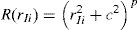
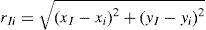
where n is the number of nodes within the influence-domain of xI, Ri (xI) is the RBF, ai(xI) and bj(xI) are non-constant coefficients of Ri(xI) and pj(xI), the polynomial basis, respectively, with m being the basis monomial number. The RBFs depend on the Euclidian distance, rIi, between the interest point xI and a node xi belonging to the ‘influence-domain’ of xI, having the following general form for a two-dimensional problem,where c and p are shape parameters that should be c=0.0001 and p=0.9999 in order to maximize the method's performance, according to the literature [32].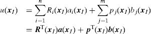
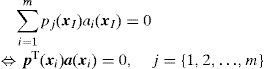
Regarding the polynomial basis functions, the purpose of adding them is to ensure the consistency of RPI functions. Notice that the literature shows that the inclusion of a RBF to the approximation functions ensures the reproducing of the linear field (C1 consistency) and improves the performance of the formulation in the patch-test [33]. Furthermore, as stated by Belinha et al. [32], the RPI does not need a polynomial basis function to pass the standard patch test. Thus, a reduction of the computational cost can be achieved, since the shape functions are only reliant on of the RBFs. Nevertheless, if it is chosen a polynomial basis with m>0, an extra requirement needs to be satisfied in order to guarantee that that the shape functions passes through the nodes,
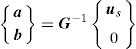
Eqs. (1) and (4) can be written in a matrix form,
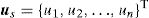
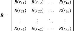
where us is given by,matrix R [n×n] in Eq. (5) is composed by the RBFs of all interest points calculated by Eq. (2),and matrix p [n×m] contains the polynomial basis functions,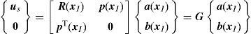
If the polynomial basis is null, in Eq. (5), R=G.
Solving Eq. (5),
Using Eqs. (5) and (9),
where φ(xI) are the interpolation functions obtained for the interest point xI.3Discrete system of equations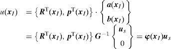
Consider a solid described by the domain Ω and boundary Γ, where Γu∪Γt=Γ, being Γu the essential boundary and Γt the natural boundary. The equilibrium equations governing the linear elasto-static problem are defined as [34],
where ∇ is the gradient operator, σ the stress tensor for a kinematically admissible displacement field u, and b the body forces per unit volume. The boundary conditions are given by σ n=t¯ on Γt and u=u¯ on Γu, where n is the outward normal to the boundary of the domain Ω, t¯ is the traction on the natural boundary Γt and u¯ is the prescribed displacement on the essential boundary Γu.
A variational form of the equilibrium Eq. (11) can be written for a generic static problem using the ‘Galerkin weak form’
being δ¿ the virtual strain tensor and δu the virtual displacement. From the Galerkin weak form, the discrete system of equations is obtained. Thus, considering the stress-strain relation, σ=c¿ (where c is the constitutive matrix), and the linear relation between strains and displacements, ¿=Lu (in which L is a differential operator that depends on the displacement field of the considered problem), Eq. (12) can be rewritten,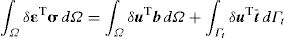

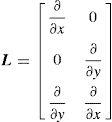
Notice that for a 2D problem the differential operator L is defined as,
Thus, the strain at an interest point xI can be interpolated with ¿(xI)=B(xI)u, where the deformation matrix B can be represented as,
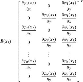
H represents blocks of diagonal matrixes, Hj, containing the shape function of each node j of a given ‘influence-domain’, with Hj=φj(xI)I, being I an identity matrix with dimension [n×n], where n is the number of degrees of freedom of the analyzed problem. For a 2D problem, it comes as,
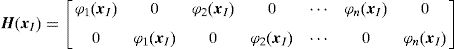
In both matrices n represents the number of nodes forming the element (in the FEM) or the number of nodes inside the influence-domain (in meshless methods).
Removing the virtual displacement δu from Eq. (13), the discrete system of equations is obtained for an elasto-static problem,
which can be written as Ku=F, with K=∫ΩBTcBdΩ and F=∫ΩH bdΩ+∫ΓH t¯ dΓ. This system of equations is the same for the FEM and meshless procedure [1]. Since the meshless method used in this work are capable to produce shape functions possessing the delta Kronecker property, the essential boundary conditions can be accurately imposed using the direct imposition method.4Micromechanical approach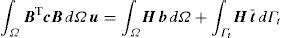
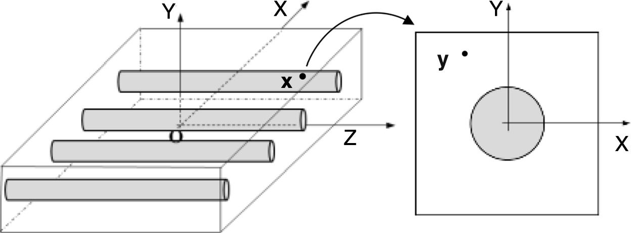
This study uses the concept of Representative Volume Element (RVE), a computational discretization concept firstly introduced by Hill [9] in 1963. The RVE is a representative sub-region [35] that statistically represents the material [3] – i.e. a sampling of all microstructural heterogeneities occurring in the composite [36]. A RVE is linked to a macroscopic point and characterizes the microstructure at that point (Fig. 2).

In this subsection, a micromechanical formulation is presented for the determination of the effective elastic properties of a composite material. Firstly, the scale transition theory is exposed, then the averaging procedure is introduced and, in the end, using periodic boundary conditions, the method to obtain the homogenized elastic properties of a composite material is fully explained.
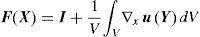
4.1Macroscopic deformation gradient and averaging theoryConsider a point at the macroscale with coordinates x which is associated to an RVE with volume V. Taking into account the microscale of that point, it can be said that there are infinitesimal points, y, belonging to the domain of the RVE placed at that macroscale point x. The notation Y defines the coordinates of a deformed point at the microscale. A perturbation of the equilibrium of the RVE can be translated to a local deformation at the macroscale point x. Thus, assuming a motion φ, the coordinates of the point x are transformed in X, such that X=φ(x). The displacement associated to that motion is given by: u(x)=φ(x)−x. Thus, it is possible to define a deformation gradient, F(x), as second-order tensor of the motion φ.
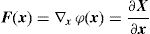
Knowing that X=x+u(x), Eq. (18) comes,
where I is the second-order identity tensor.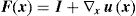
Using a homogenization procedure, a macroscopic deformation gradient, F(X) can be determined through the correspondent microscopic deformation gradients,
where the microscopic deformation gradient, F(Y), can be expressed as,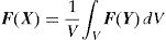
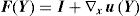
Thus,
If one applies a macroscale deformation gradient at the point x (i.e. to a RVE), a microscopic displacement field is produced and it is given by Eq. (23).

which has a linear part depending on the prescribed deformation gradient, F(X), and a displacement fluctuation, u˜ (Y), an unknown variable of the microscopic equilibrium problem.
According to Eq. (23), the imposition of a specific macroscale deformation gradient to the RVE, allows to obtain the microscopic displacement field. Consequentially, the stress and strain fields installed in each integration point of the RVE can be obtained and then homogenized through the volume V of the RVE. Thus, the macroscale stress, σ¯, and strain, ε¯, tensor at the point X are derived by averaging the stress and strain tensor over the volume of the RVE,

Thus, the homogeneous medium of a composite given by the average stresses, strains and also the effective elastic constants is equivalent to the actual heterogeneous medium [37], as stated by the Hill–Mandel principle using energy considerations.
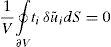
4.2Hill–Mandel principleThe Hill–Mandel principle establishes a relationship between the two scales. It states that if the sub-scale-modelling is energetically consistent, the deformation energy at the macroscopic level should be equal to the volume average of micro-scale stress work [38]. Thus, the principle is represented by Eq. (25),
which, after mathematical manipulation, considering δεij=δε¯ij+δε˜ij and 1V∫Vσij δε˜ij dV=0, and using the Gauss Theorem, becomes,being ti an external traction. In Eq. (26) is considered the absence of body forces.4.3Periodic boundary conditions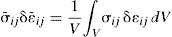
The boundary conditions of RVE for the displacement and the traction fields should be defined in order to satisfy Eq. (26). In the literature are found several types of boundary conditions imposed on RVEs, such as the linear displacement boundary condition (Dirichlet condition which assumes the displacement fluctuation field is null), uniform traction boundary conditions (Neumann condition) or periodic boundary conditions. The periodic boundary conditions (PBCs) satisfy the Hill–Mandel principle and are stated in many numerical studies as the most efficient in terms of convergence rate [38]. Consequently, this type of boundary conditions are adopted in this work.
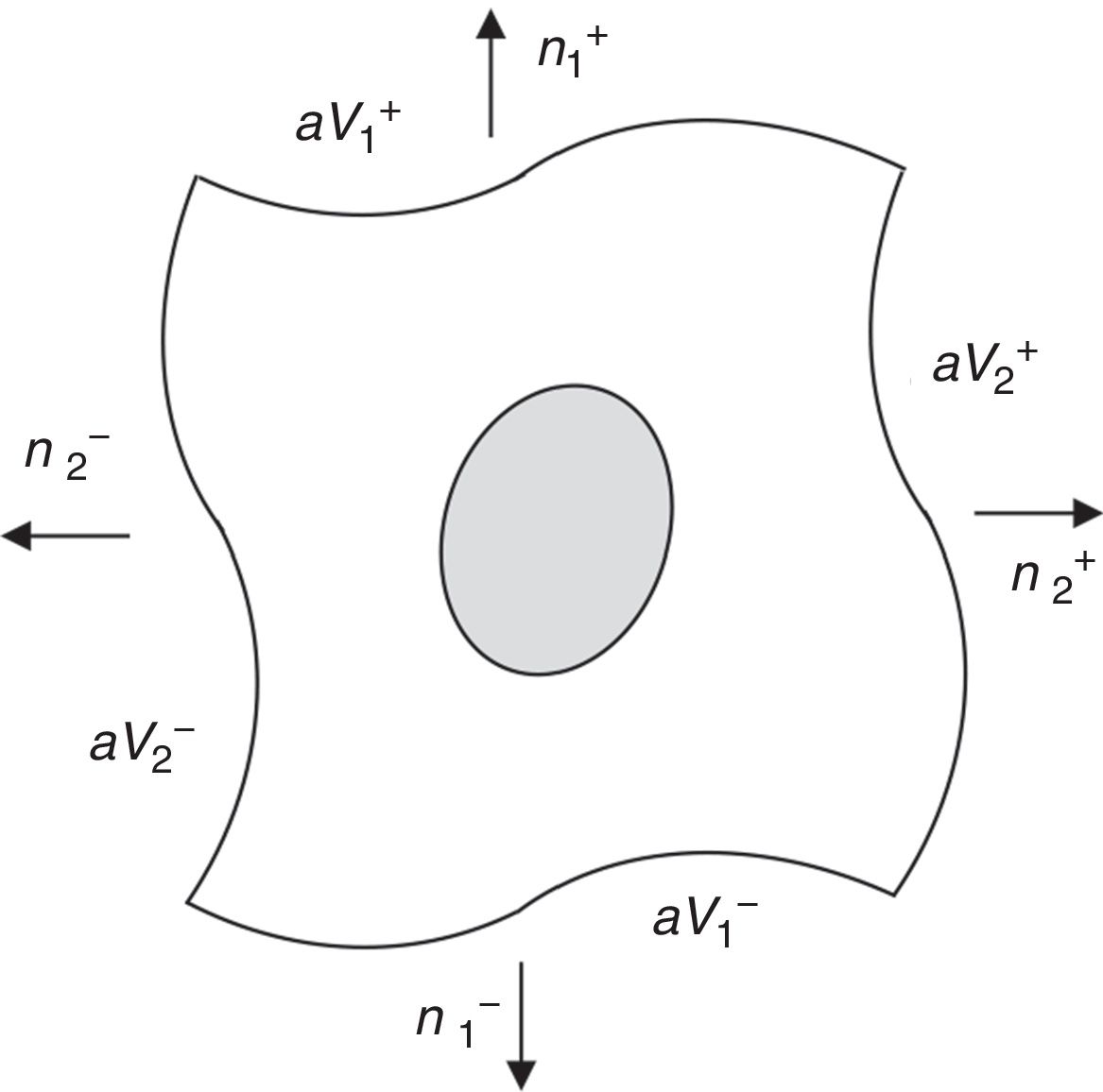
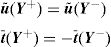
To impose PBCs on a RVE, the displacement fluctuation fields on opposite boundaries of the RVE must be periodically equal, while the distribution of the traction field must be anti-periodic on those opposite boundaries of the RVE. Thus, for a RVE with boundary ∂V, consider its positive, ∂V+, and negative, ∂V−, part, such that ∂V=∂V+∪∂V− (Fig. 3).

The outward normal to the boundaries represented in Fig. 3 are symmetric, n+=−n−, at Y+∈∂V+ and Y−∈∂V−. Thus, PBCs can be expressed using Eq. (27),
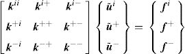
Thus, in order to apply these boundary conditions directly in the stiffness matrix defined in Section 3, the displacement fluctuation field can be usefully divided into three parts:
being u˜i the displacement fluctuation of the inner nodes of the RVE and u˜+ and u˜− represent the displacement fluctuation of the positive and negative boundaries of the RVE, respectively. Based on this assumption, the discrete system of equations can be rewritten in the following form,
Thus, according to the space of admissible displacement fluctuations, the condition u˜+=u˜− is forced using, for instance, the Gauss elimination method. The condition f+=−f− is imposed on the vector of the second member of Eq. (29).
Additionally, in order to prevent rigid body motions, in this work the displacements at the corners of the RVE were constrained.
4.4Determination of the homogenized elastic propertiesThis study uses a numerical procedure that consists on applying different strain states (pure strain and pure shear deformation) to a RVE. Using these well-defined strain fields, homogenized stress fields are obtained and, using the Hooke's law, the effective elastic constants are obtained.
Two-dimensional RVEs were considered in a plane-strain state since the longitudinal length of the fibres in a composite laminate is much larger than the dimensions of their cross section dimensions. The plane strain state considers that the dimension of the solid along the z direction is much larger than its other dimensions, therefore ¿zz=¿zy=¿zx=0, but σzz≠0.
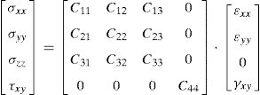
Consider the Cauchy stress tensor given by Eq. (30)
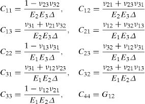
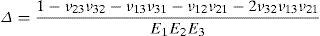
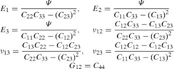
and the constitutive equation, with the stress and strain tensors written in the Voigt notation,where the constants presented in the constitutive matrix are given as,with,where E1 and E2 are the Young modulus along the transverse directions of the fibres (the directions of the plane), E3 is the Young modulus along the fibres direction (longitudinal direction – normal direction to the plane), υij is the Poisson ratio which characterizes the deformation rate in direction j when a force is applied in direction i, Gij is the shear modulus which characterizes the variation angle between directions i and j. The elastic properties can be written as a function of the matrix components, Cij,where Ψ is given by,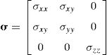

The procedure to obtain the homogenized elastic properties of a fibre composite material can be summarized in the following steps,
- (a)
Applying macroscopic deformation gradients to a RVE producing two pure strain and one shear deformation state (for a 2D problem).
- (b)
Imposing periodic boundary conditions and solving the boundary problem.
- (c)
Determination of the stress field in each integration point of the RVE.
- (d)
Numerical homogenization of the stresses.
- (e)
Determination of the constants Cij using the Hooke's law.
- (f)
Determination of the elastic properties using the relations (34).
For instance, consider an imposed deformation gradient on the RVE, such that ¿xx=1 and the other components of the strain tensor are null. Using Eq. (31), the following expressions are found,

If ¿yy=1 and the other components of the strain are null, one achieves:

Using a third deformation gradient producing a pure shear strain field (¿xx=¿yy=0 and γxy=1), it is obtained,

Through this procedure, only one elastic constant cannot be obtained, C33. To solve this problem, the longitudinal Young modulus is approximated using the rule of mixtures (ROM),
being Vf the volume fraction of fibres in the composite laminate. Knowing E3*, C33 can be obtained, leading to the determination of all elastic properties – Eq. (34).5Numerical examples
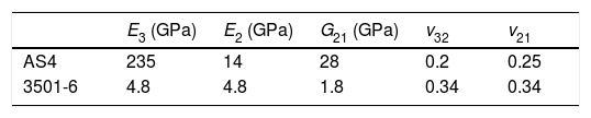
Using the formulations presented in the previous sections, numerical results were obtained for the effective elastic properties of a composite material (unidirectional graphite fibre – AS4 – as reinforcement phase and epoxy – 3501-6 – as matrix phase). In this study, the fibre is considered as an anisotropic and homogeneous material, while matrix material is considered isotropic and homogeneous, with the elastic properties shown in Table 1[37].
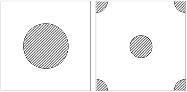
In a real unidirectional fibre-reinforced composite, the arrangement of fibres is random. Thus, due to the difficulty to model its geometry, simplified RVEs with non-periodic distribution of fibres were considered (Fig. 4).
 square – Type 1 – and (b) hexagonal arrays – Type 2.")
In the following subsections, convergence and computation time studies will be presented concerning these two arrays of RVEs and two numerical approaches (the RPIM and the Finite Element Method with quadrilateral linear elements) and, after that, a benchmark problem is analyzed, being the obtained results compared with the available solutions found in literature.
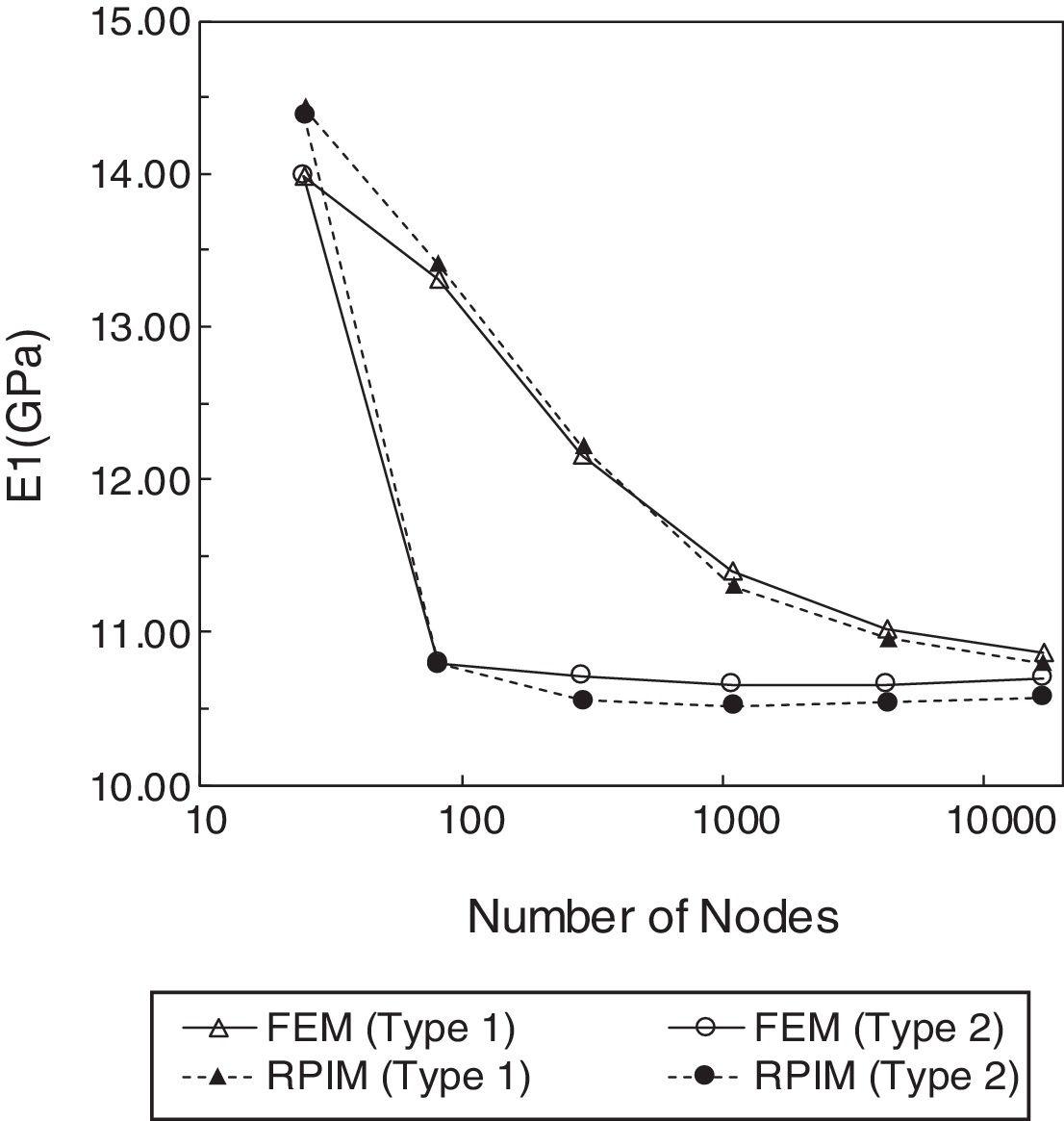
5.1Convergence and computation time studiesThe material of Table 1 with a volume fraction of fibres of Vf=0.6 was considered. The homogenized transverse Young modulus (in-plane direction) of the composite material is obtained for nodal meshes with an increasing number of nodes (from 25 to 16641 nodes). In the RPIM are considered fixed size influence-domains with 16 nodes per integration point. In the FEM formulation, it is used exactly the same number of nodes as the nodal mesh of the RPIM (and the same Gaussian integration mesh is also adopted), but the nodal connectivity is ensured, in this case, by the interaction of adjacent elements rather than an overlap rule of influence-domains. The convergence studies using the Type 1 and Type 2 RVEs are presented in Fig. 5. By observation of those graphs, it can be concluded that the FEM and the RPIM have similar convergence paths, despite FEM achieves convergence slightly faster. Another conclusion that can be taken from the graph of Fig. 5 is that the configuration of the RVE considerably affects the convergence rate of the solution – the hexagonal array converges faster than a square array. In the end, meshes with 65×65 nodes were selected for further analysis.

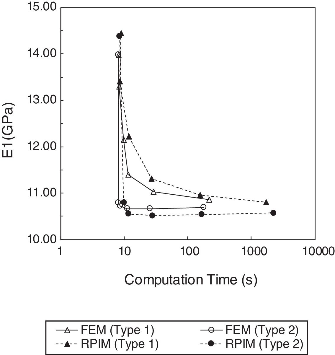
Regarding the time consumed by both numerical techniques (Fig. 6), it can be concluded that, due to the more complex nodal connectivity, the RPIM is computational more expensive than the FEM, when comparing the computation time related to the same nodal mesh. Nevertheless, for a given computation time (in seconds), the RPIM obtains a lower value for the transverse Young modulus, in both RVE arrays, leading to a more accurate solution, as it will be shown in the next subsection.
5.2Benchmark example
In this subsection, the material of Table 1 was considered using 0.6 of fibre volume fraction. The meshless and FEM solutions were compared with solutions from the literature [37] and also with the elastic properties provided by the rule of mixtures (ROM), which states that,
being the indexes (·)f and (·)m related to the properties of the fibre and the matrix, respectively.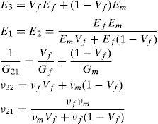
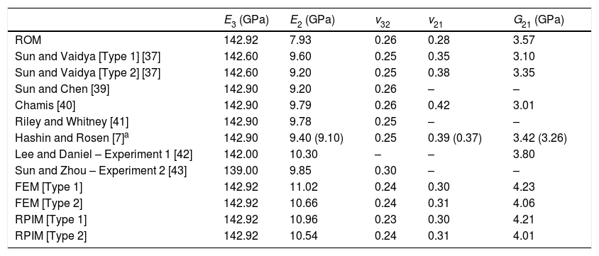
In Table 2 are presented the solutions for the longitudinal Young modulus, transverse Young modulus, out-of-plane Poisson coefficient, in-plane Poisson coefficient and in-plane shear modulus. Sun and Vaidya [37] are 3D FEM solutions, Sun and Chen [39] and Chamis [40] presented solutions based on a mechanics approach involving the use of displacement continuity and force equilibrium conditions. Hashin and Rosen [7] solutions are analytical results based on energy variational principles while Riley and Whitney's [41] solution is based on the use of the energy balance approach with the aid of classical elasticity theory. The other two literature solutions presented in Table 2 are based on experiments.
Effective elastic properties for AS4/3501-6 composite (Vf=0.6).
| E3 (GPa) | E2 (GPa) | v32 | v21 | G21 (GPa) | |
|---|---|---|---|---|---|
| ROM | 142.92 | 7.93 | 0.26 | 0.28 | 3.57 |
| Sun and Vaidya [Type 1] [37] | 142.60 | 9.60 | 0.25 | 0.35 | 3.10 |
| Sun and Vaidya [Type 2] [37] | 142.60 | 9.20 | 0.25 | 0.38 | 3.35 |
| Sun and Chen [39] | 142.90 | 9.20 | 0.26 | – | – |
| Chamis [40] | 142.90 | 9.79 | 0.26 | 0.42 | 3.01 |
| Riley and Whitney [41] | 142.90 | 9.78 | 0.25 | – | – |
| Hashin and Rosen [7]a | 142.90 | 9.40 (9.10) | 0.25 | 0.39 (0.37) | 3.42 (3.26) |
| Lee and Daniel – Experiment 1 [42] | 142.00 | 10.30 | – | – | 3.80 |
| Sun and Zhou – Experiment 2 [43] | 139.00 | 9.85 | 0.30 | – | – |
| FEM [Type 1] | 142.92 | 11.02 | 0.24 | 0.30 | 4.23 |
| FEM [Type 2] | 142.92 | 10.66 | 0.24 | 0.31 | 4.06 |
| RPIM [Type 1] | 142.92 | 10.96 | 0.23 | 0.30 | 4.21 |
| RPIM [Type 2] | 142.92 | 10.54 | 0.24 | 0.31 | 4.01 |
The numerical results obtained proved to be close to the solutions from the literature, allowing the validation of the algorithm developed for heterogeneous materials. Since the solutions from the literature present a certain range (for instance, the effective transverse Young modulus varies between 9.10 and 10.30GPa), the present solutions fit the magnitudes expected.
When comparing the RPIM with the FEM solutions, it can be said that the RPIM solutions are always closer to the literature solutions. Even though both numerical approaches use the same nodal and integration meshes, the way the nodal connectivity is imposed and the field variables are approximated allows to obtain distinct solutions.
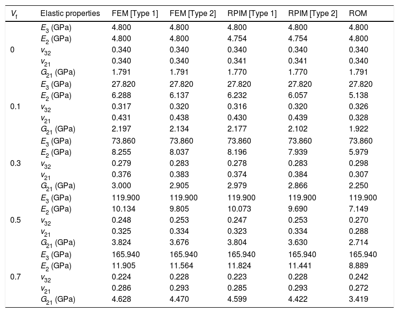
5.3Effect of the volume fraction of fibres on elastic propertiesIn this subsection, the effect of the volume fraction of fibres on elastic properties is investigated. Using the same constituents of Table 1, RPIM and FEM solutions are found for different fibre volume fractions, without exceeding the maximum value of Vf,
being L and D the dimensions of the RVE.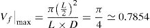
In Table 3 are shown the numerical solutions and the ROM solutions for comparison purposes. For Vf=0, it is obtained the elastic properties of the matrix given in Table 1, as was expected.
Effective elastic properties for AS4/3501-6 composite using different fibre volume fractions.
| Vf | Elastic properties | FEM [Type 1] | FEM [Type 2] | RPIM [Type 1] | RPIM [Type 2] | ROM |
|---|---|---|---|---|---|---|
| 0 | E3 (GPa) | 4.800 | 4.800 | 4.800 | 4.800 | 4.800 |
| E2 (GPa) | 4.800 | 4.800 | 4.754 | 4.754 | 4.800 | |
| v32 | 0.340 | 0.340 | 0.340 | 0.340 | 0.340 | |
| v21 | 0.340 | 0.340 | 0.341 | 0.341 | 0.340 | |
| G21 (GPa) | 1.791 | 1.791 | 1.770 | 1.770 | 1.791 | |
| 0.1 | E3 (GPa) | 27.820 | 27.820 | 27.820 | 27.820 | 27.820 |
| E2 (GPa) | 6.288 | 6.137 | 6.232 | 6.057 | 5.138 | |
| v32 | 0.317 | 0.320 | 0.316 | 0.320 | 0.326 | |
| v21 | 0.431 | 0.438 | 0.430 | 0.439 | 0.328 | |
| G21 (GPa) | 2.197 | 2.134 | 2.177 | 2.102 | 1.922 | |
| 0.3 | E3 (GPa) | 73.860 | 73.860 | 73.860 | 73.860 | 73.860 |
| E2 (GPa) | 8.255 | 8.037 | 8.196 | 7.939 | 5.979 | |
| v32 | 0.279 | 0.283 | 0.278 | 0.283 | 0.298 | |
| v21 | 0.376 | 0.383 | 0.374 | 0.384 | 0.307 | |
| G21 (GPa) | 3.000 | 2.905 | 2.979 | 2.866 | 2.250 | |
| 0.5 | E3 (GPa) | 119.900 | 119.900 | 119.900 | 119.900 | 119.900 |
| E2 (GPa) | 10.134 | 9.805 | 10.073 | 9.690 | 7.149 | |
| v32 | 0.248 | 0.253 | 0.247 | 0.253 | 0.270 | |
| v21 | 0.325 | 0.334 | 0.323 | 0.334 | 0.288 | |
| G21 (GPa) | 3.824 | 3.676 | 3.804 | 3.630 | 2.714 | |
| 0.7 | E3 (GPa) | 165.940 | 165.940 | 165.940 | 165.940 | 165.940 |
| E2 (GPa) | 11.905 | 11.564 | 11.824 | 11.441 | 8.889 | |
| v32 | 0.224 | 0.228 | 0.223 | 0.228 | 0.242 | |
| v21 | 0.286 | 0.293 | 0.285 | 0.293 | 0.272 | |
| G21 (GPa) | 4.628 | 4.470 | 4.599 | 4.422 | 3.419 | |
The transverse Young modulus characterizes the response of the material to the application of a load in the perpendicular to the fibres direction. An increase of the fibre volume fraction increases the transverse modulus of the studied composite, as it is suggested by the ROM (the stiffness of the fibre becomes more predominant). This fact is well captured by the numerical solutions.
In the case of the Poisson's ratio, it can be seen a good agreement between the numerical homogenized solutions and the ROM solutions for the out-of-plane Poisson's ratio, but the same does not happen for the in-plane Poisson's ratio, which seems to be overestimated for lower values of the fibre volume fraction of fibres.
6ConclusionsUsing the Finite Element Method and the Radial Point Interpolation Method as discretization techniques, this work proposes a computational homogenization approach for the determination of the effective elastic properties of a heterogeneous material. The micromechanic approach used in this work was based on the assumption that the solids under study were submitted to a 2D plane strain state. That consideration allowed to study fibre composite materials in a simplified way, reducing the computational effort due to the reduction of the number of degrees of freedom of the problem.
The algorithms developed were successfully validated using a benchmark example and it was verified that, in general, the effect of the fibre volume fraction on a fibre composite material is well captured by the numerical techniques.
The developed computational tool is now able to analyze any kind of microstructures with several heterogeneities and periodicity, only being necessary to know the material properties of its constituents. This micromechanical numerical tool can also be coupled with a macroscale analysis in a multi-scale framework, creating a more accurate way to evaluate the local elastic properties on the integration points of the macroscale analysis.
Regarding the meshless method studied, this work shows that, using the exactly same nodal and integration meshes of the FEM, the RPIM can achieve slightly more accurate results. Thus, it is possible to conclude that RPIM is a robust and accurate numerical tool, constituting as a strong alternative to the traditional FEM, whose use has become widespread in the field of engineering design.
The authors truly acknowledge the funding provided by Ministério da Ciência, Tecnologia e Ensino Superior – Fundação para a Ciência e a Tecnologia (Portugal), under grants: SFRH/BPD/111020/2015 and SFRH/BD/121019/2016, and by project funding MIT-EXPL/ISF/0084/2017 and UID/EMS/50022/2013 (funding provided by the inter-institutional projects from LAETA). Additionally, the authors gratefully acknowledge the funding of Project NORTE-01-0145-FEDER-000022 – SciTech – Science and Technology for Competitive and Sustainable Industries, co-financed by Programa Operacional Regional do Norte (NORTE2020), through Fundo Europeu de Desenvolvimento Regional (FEDER).
The author truly acknowledge the work conditions provided by the Department of Mechanical Engineering from FEUP and INEGI.
