

Maximum-minimum bidirectional options are a kind of exotic path dependent options. In the constant elasticity of variance (CEV) model, a combining trinomial tree was structured to approximate the non-constant volatility that is a function of the underlying asset. On this basis, a simple and efficient recursive algorithm was developed to compute the risk-neutral probability of each different node for the underlying asset reaching a maximum or minimum price and the total number of maxima (minima) in the trinomial tree. With help of it, the computational problems can be effectively solved arising from the inherent complexities of different types of maximum-minimum bidirectional options when the underlying asset evolves as the trinomial CEV model. Numerical results demonstrate the validity and the convergence of the approach mentioned above for the different parameter values set in the trinomial CEV model.
Las opciones bidireccionales máximas-mínimas son un tipo de opciones exóticas dependientes de la trayectoria. En el modelo de elasticidad constante de la varianza (ECV), se estructuró un árbol trinomial combinado para aproximar la volatilidad no constante, que es una función del activo subyacente. En base a esto se desarrolló un algoritmo sencillo y eficaz para calcular la probabilidad de neutralidad al riesgo de cada nodo del activo subyacente llegando a un precio máximo o mínimo y el número total de máximos (mínimos) del árbol trinomial. De esta manera, los problemas computacionales pueden resolverse eficazmente a raíz de las complejidades inherentes a los distintos tipos de opciones bidireccionales máximas-mínimas cuando el activo subyacente evoluciona como el modelo ECV trinomial. Los resultados numéricos demuestran la validez y convergencia del enfoque anteriormente mencionado para los parámetros de valores establecidos en el modelo ECV trinomial.
Black and Scholes (1973) derived the well-known option pricing formula by assuming the underlying asset price follows a geometric Brownian motion. Under the construction, the price distribution is lognormal and volatility is constant. However, in the market reality, where often the asset price behavior is affected by volatility smile effect, this implies that the asset price is generally unlikely to be lognormally distributed the underlying asset volatility tends to change as asset price moves up and down. Cox (1975) initially observed that the character of the volatility of the underlying asset was linked to its price level. He noted that the origin of the volatility smile was the negative correlation between asset price changes and volatility changes, on this basis Cox developed constant elasticity of variance (CEV) model. As documented by Beckers (1980) and Davil (1982), there are theoretical arguments for and empirical evidences for the validity of CEV model. Many empirical studies in Macbeth and Merville, 1980 and Emanuel Macheth (1982) have shown that CEV model better describe the evolution of asset price. Hence it is instructive to apply CEV model to option pricing.
The problem of pricing a standard European option, when the underlying asset value is driven by a CEV model was solved by Cox and Ross (1976) who derived an analytical solution for the option value. Things are more complicated in the case of path-dependent options. The analytical solution of the pricing problem is not available and numerical approximations must be used. Boyle and Tian (1999) used Monte Carlo simulations. Subsequently, he extended Babbs method on the basis of Black-Scholes model to construct a trinomial tree method for evaluating the lookback options under the CEV model, as was translated into Chinese by He (2001). Duvydov and Linetsky (2001) derived the close-form formulae of barrier options under the CEV model with help of the numerical inversion of the Laplace transform of the option price following ordinary differential equation. Bin and Fei (2006) applied the intuition binomials tree method to price Asian option under the constant elasticity of variance. Among these numerical techniques, trinomial tree evaluation approach still plays a remarkable role both for its highly flexible and implementation in solving the pricing problem of path-dependent options under the CEV model. However, in the framework of the trinomial tree to approximate the constant elasticity of variance model, the transition probabilities are no longer constant over the tree. This property introduces a further complication in the evaluation process. In addition, there is little work on the exotic path-dependent such as maximum-minimum bidirectional options.
The objective of this paper is to study the application of the trinomial tree approach to maximum-minimum bidirectional options when the asset price evolves as a CEV model. Especially, recursive algorithm based on a forward induction procedure is developed to compute the risk-neutral probability of each different node for the underlying asset reaching a maximum or minimum price in the binomial tree. The remainder of the paper is organized as follows: Section 2 illustrates the trinomial method used to approximate the CEV model under the equivalent martingale measure. In Section 3 the trinomial approximation is applied to price maximum and minimum bidirectional options and numerical results are given. Conclusions are presented in the final section.
2A trinomial CEV modelIt is known that Black-Scholes model with constant volatility does not hold empirically for asset prices. Alternative stochastic models have been studied and applied to option pricing. For example, Cox (1975) and Davil (1982) study a general class of stochastic model known as the Constant Elasticity of Variance (CEV) diffusion model in a risk-neutral world.
where B is a standard Wiener process under the Q-measure, r is riskless rate of interest, the standard deviation of return σ is a function of the underlying price instead of a constant δ and a are constants, 0≤a<2.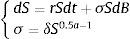
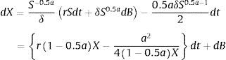
We consider a discrete approximation for the asset price evolution described in (1) using the trinomial approach. Let n be the number of time intervals between the time t and the maturity T, [t,T] is divided into n equal pieces, each of width Δt. The underlying asset may move up a level, down a level or stay the level with geometric average between up level and down level. In the case of the asset price dynamics driven by CEV model, the volatility is not a constant but varies with the level of the underlying price. This implies that the approximation trinomial tree is non-recombining and the number of nodes produced at each vertical layer is 3ii=0…….n, thus computational complexity becomes unmanageable even with a small number of time steps. In order to effectively solve the computational problems arising from the inherent complexities of the constant elasticity of variance model, we need to transform the variable S governed by (1) with non-constant volatility so that the transformed process has constant volatility. Considering the transformed process Xt=S1−0.5a/(1−0.5a)δ and using the Ito's Lemma, we have:
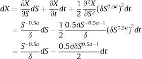
Substituting equation (1) into the above equation and using the fact that S=δ1−0.5aX1/1−0.5a. Equation (2) becomes:
Now, it is easy to build up a computationally simple trinomial tree to approximate the X-process. The value Xt of the process at time t, after one period at time t+1, can rise to Xt+Δt, or decrease to Xt−Δt, or stay the same with Xt. Continuing in this way, we see that the value of the trinomial X-process are equal to

Where Xt+iΔtj represents the value of the trinomial X-process at time t+iΔt after j/2 up steps and i-j/2 down steps. for i=0,1,….,n and j=0,1,….,2i.
Given the values on the X lattice, we can recover the dynamics of the underlying price on its lattice. As before, consider the value Stj of the process at time t, after one period at time t+1, can rise to St+i1tj+=f(Xtt+Δt), or decrease to St+i1tj−=f(Xtt−Δt), or stay the same with St. Continuing in this way, we note that the value of the binomial approximating S-process at time t+iΔt after j/2 up steps and i-j/2 down steps. is expressed as follows:

Once we have developed the trinomial tree that approximates the S-process, it remains to compute the probabilities of an upward and downward move for the evolution of the asset price in the approximating trinomial tree. To ensure non-negative and less than one probabilities, it is optimal to have the underlying asset price of central move equivalent to the expected asset price of the underlying stochastic process we define St+iΔtj¯, j=0,1,…2i to be greatest with up jumps such that erΔtSt+(i-1)Δtj=St+iΔtj¯<0 with up probability pt+(i-1)Δtj and St+iΔtjˆ to be the smallest with down jumps such that erΔtSt+(i−1)Δtj−St+iΔtjˆ>0. with down probability qt+(i−1)Δtj and St+iΔtj˜ to be middle move between the greatest and the smallest, such that erΔtSt+(i-1)Δtj−St+iΔtj˜=0.
The probabilities that the underlying asset with price St+(i−1)Δtj makes an up jump and down jump are specified by the following set of equation,
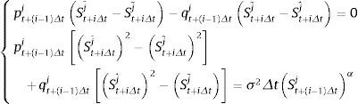
Solving for the probabilities from the above equation, one obtain:
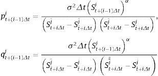
Obviously, the probability that the underlying asset with price St+(i−1)Δtj makes parallel move is 1−pt+(i−1)Δtj−qt+(i−1)Δtj. The above calculation of the transition probabilities pt+(i−1)Δtj and qt+(i−1)Δtj represents legitimate probabilities which allows for multiple jumps in the approximating trinomial X-process. This is important because, in the region near to S=0, the magnitude of each jump could be very small and, as a consequence, the transition probabilities could exceed one or smaller than zero.
3Pricing maximum-minimum bidirectional optionsWe now apply the trinomial CEV model depicted in above section to pricing the maximum-minimum bidirectional options Invoking the no-arbitrage principle, the value at time t of options is given by discounting at the risk-free interest rate the sum of all the option payoffs multiplied by the corresponding probability of occurring. Thus we need to see the .payoff corresponding to each node of the tree at maturity. For floating striking maximum-minimum bidirectional options, its payoff at maturity is equal to the difference between the current underlying asset and the minimum price registered by the underlying asset during the option life time plus the difference between the maximum underlying asst price registered during the option life time and current asset price. Conversely, the fixed strike maximum-minimum bidirectional options pay off the maximum between zero and the difference between the maximum underlying asset price and a fixed strike price plus the maximum between zero and the difference between a fixed strike price and the minimum asset price. However, things are complicated by the fact that, to each terminal node of the tree correspond, in general, different values of the option payoff. This is because, even when some trajectories of the underlying asset price end with the same terminal value, they could have registered a different minimum and maximum price during the option lifetime.
In the framework of the trinomial CEV model developed by Section 2 we see that the transition probabilities are not constant over the tree, and as a consequence, all the paths of the underlying asset with the same terminal value may have the different probabilities of occurring. In this framework, the evaluation problem is not solved even if we can compute the number of paths with the same terminal value but with a different minimum or maximum price registered during the option life. This property introduces a further complication in the evaluation process. To copy with this problem, we derive a recursive algorithm based on a forward induction procedure that allows to simply compute the risk-neutral probability of each different payoff of the options at maturity. The algorithm works as follows: at first, we write (i, i-j) for the trinomial lattice where the underlying asset has a price St+iΔtj (i=0,1,….,n; j=0,1,….,2i). Note that i-j is the difference between the down steps and the up steps taken by the underlying asset price and, as we see below, it is useful representation of position of the asset price at time i. Further, we use index k and h (k, h=0,1,….i) respectively to specify the lowest and highest layer of horizontal nodes reached by the underlying asset price after i time steps. In other words, k=0,1,….i means that the asset with current price St+iΔtj has registered minimum price equal to St+kΔt0, h=0,1,….i means that the asset with current price St+iΔtj has registered maximum price equal to St+hΔt2h we use the triplet (i,j, k) and (i,j, h) to respectively specify the state of the world in which the underlying asset reached a minimum price equal to St+kΔt0 and a maximum price equal to St+hΔt2h,. over a path with j/2 up steps and i-j/2 down steps. Clearly, given i and j, the value of the index k ranges over the internal maxi−j,0,i−j/2; and the value of the index h ranges over the internal maxj−i,0,j/2, where ∘ returns the lower integer is closest to a real number. With help of these important relations, we can identify all the different minimum prices, St+kΔt0 and all the different maximum prices, St+hΔt2h registered by the underlying asset price that has a current value St+iΔtj.
We start by computing the probability of each state of nature represented by the triplet (i,j, k) in the trinomial tree. To do this, we need to distinguish two cases, the first considers the states of nature characterized by the triplet (i, j, k) such that k=i-j. In this case the underlying asset price was at the node (i,i−j),St+iΔtj is located on the same horizontal set of nodes of the minimum price reached by the underlying asset during the first time steps. This means that at time t+(i−1)Δt the underlying asset price was at the node (i−1,i−1−j) and the last step from (i−1,i−1−j) to (i,i−j) is a down step. If at time t+(i−1)Δt the underlying asset price was at node (i−1,i−1−(j−1)) the lowest layer of nodes reached by the underlying asset price would be located at the level k=i−j and this is equivalent to the hypothesis k=i−j. this means the underlying asset could reach the minimum price St+kΔt0 at time t+iΔt with the last parallel move. Hence the state of nature (,i,j,k) is:
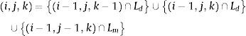
Where Ld and Lmrespectively represents the event that the last time step taken by the underlying asset price is a down step and stay the same. Hence, the probability of the state of nature (,i,j,k) is
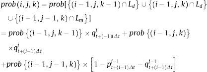
The second case considers the states of nature such that k>i−j. in this situation the underlying asset price at the node (i,i−j),St+iΔtj is greater than the minimum price reached during the first i−1 time steps. Indeed, the lowest layer of nodes touched by the underlying asset is located at level k, that is, below the current node (i,i−j) located at level i−j. in this situation, the level k was already reached by the underlying asset price at time t+(i−1)Δt. If the asset price is at the node (i−1,i−1−j) and the ith step is a down step and if the asset price is at the node (i−1,i−1−(j−1)) and the ith step is parallel step and if the asset price is at the node (i−1,i−1−(j−2)) and the ith step is an up step. Thus the event (i,j,k) occurs when the event (i−1,j,k) occurs and the ith step is a down step or when the event (i−1,j−1,k) takes place and the ith step is parallel step or when the event (i−1,j−2,k) takes place and the ith step is an up step, i.e.
where Lu represents the event that the last step taken by the underlying asset price is an up step. Hence, the probability of the state of nature (i,j,k) is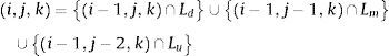
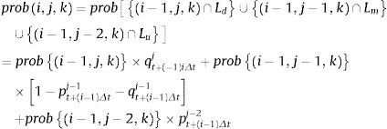
The case of the probability of each state of nature represented by the triplet (i, j, h) in the trinomial tree can be computed as before. We must distinguish between two cases, the first is when the current price of the underlying asset, St+iΔtj is equal to the maximum value of the asset price, i.e. h= j-.i. In this case the last step of the asset price must be an up step or parallel step and maximum may be reached with the last time step or during the first i-1 time steps. Hence,
and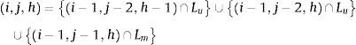
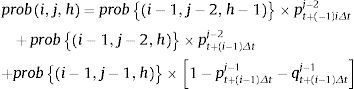
On the contrary, when the maximum underlying asset price is greater than the current asset price, i.e. h>j−.i, we have
and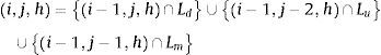

It is worth noting that the recursive algorithm for computing the risk neutral probability of each state of nature at the beginning of the tree, assigns the risk-neutral probability 1 to the state of nature (0,0,0) and a risk-neutral probability 0 to the states of natures that can never occur, i.e, when k<0 or k>i−j/2i−j/2 and h<0 or h>j/2.
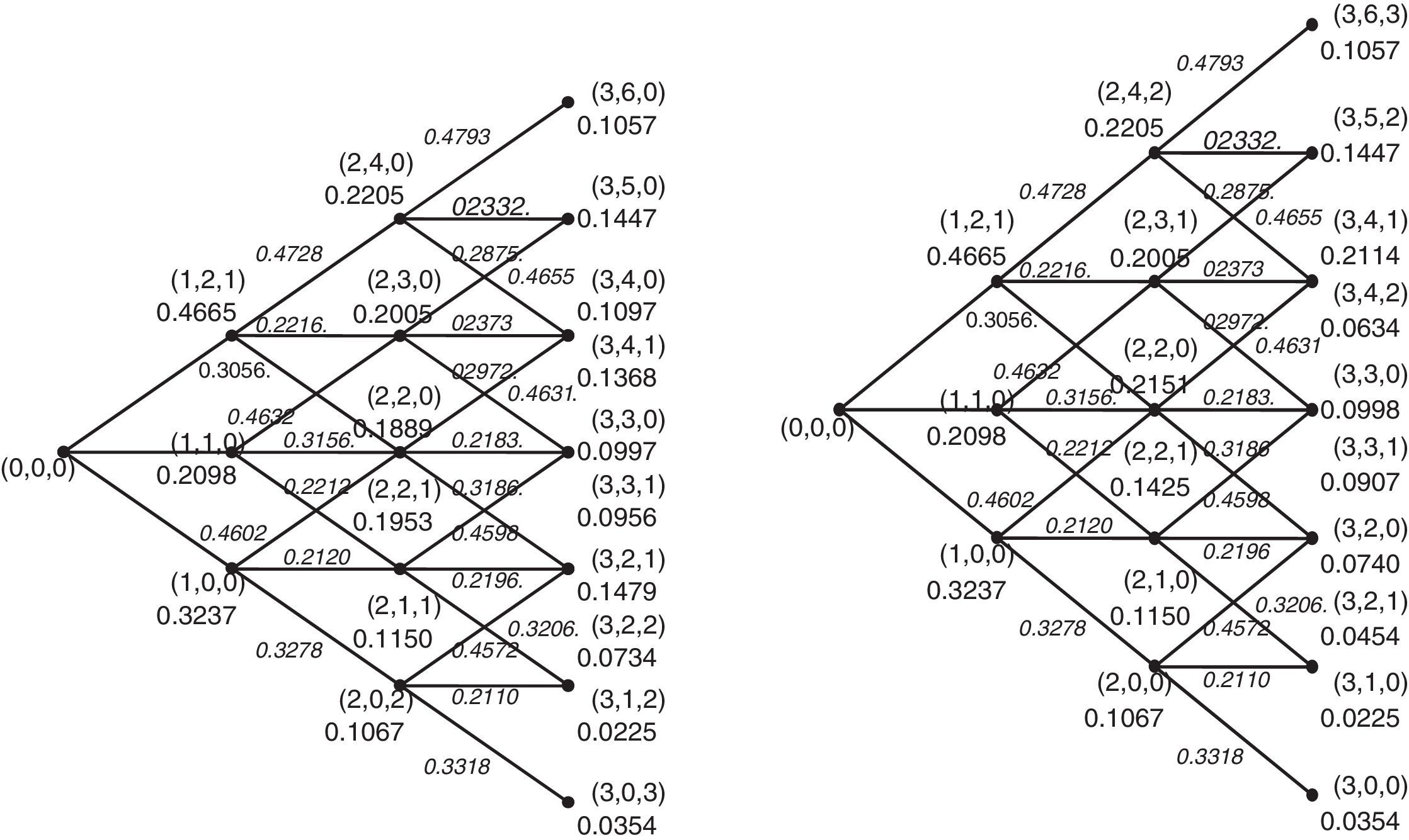
To clarify how the procedure works we consider asset with price St=100 that moves in the trinomial lattice illustrated in Section 2. We consider the number of time steps n=3, the risk=free interest rate r=10%, the time to maturity T=6 months and elasticity factor a=05. the volatility parameter σis adjusted in such a way that the instantaneous volatility of the asset price at inception is the same for all the values of the parameter a considered. We set the initial instaneous volatility of the underlying asset rate of return equal to 0.25 and select the value of σ such that δSta/2−1=0.25.
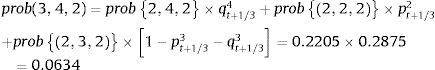
Figure 1 illustrates how the forward induction based procedure works in computing the risk neutral probability of each minimum and maximum in the trinomial tree. In the Figure 1, we depict the trinomial tree that describes the evolution of the underlying asset price and we reported the risk-neutral probability of each up step and of each down step and middle step. For example, 0.4572 is the probability, pt+1/30 that the underlying asset price jumps from the value ST+1/30 to the price St+1/22 represented by the node (3,2). The left hand side of Figure 1 illustrates the risk-neutral probability of each possible minimum reached by the underlying asset that currently is located at the node (i, i-j). For example, at the node (3,2), the underlying asset price has a current price St+1/22. The minimum price reached by the underlying asset price if the first or second step was an down step is St+1/60, hence k=1 and the state of nature occurred is (3,2,1) because i−j=k, prob(3,2,1)=[prob2,2,0+prob2,2,1]×qt+1/32+prob2,1,1×1−pt+1/31−qt+1/31=0.1889+0.1953×0.3186+0.1150×0.2196=0.1479
 and (i,j,h).")
Conversely, in the case of two consecutive down steps of the underlying asset price at inception, the minimum price reached by the underlying asset price is St+1/30, k=2, and the state of nature occurred is (3,2,2). Because k>i−j
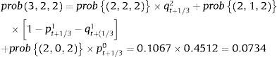
Note that the state of nature (2,2,2) and (2,1,2) can never occur.
The right hand side of Figure 1 illustrates the risk-neutral probability of each possible maximum reached by the underlying asset that currently is located at the node (i,i−j). For instance, at the node (3,4), the underlying asset price has a current price St+1/24. The maximum price reached by the underlying asset price if the first or second step was an up step is St+1/62, hence h=1 and the state of nature occurred is (3,2,1) because j−i=h, prob3,4,1=prob2,2,0+prob2,2,1×pt+1/32+prob2,3,1×1−pt+1/33−qt+1/33=(0.2151+0.1425)×0.4631+0.2005×0.2313=0.2114
On the contrary, in the case of two consecutive up steps of the underlying asset price at inception, the maximum price reached by the underlying asset price is St+1/34,h=2, and the state of nature occurred is (3,4,2). Because h>j−i
Note that the state of nature (2,2,2) and (2,3,2) can never occur.
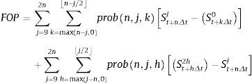
Once we compute the risk-neutral probability of eaxh state of nature at maturity, (n,j,k) and (n,j,h), j=0,1,….2n, k=maxi−j,0,.......i−j/2h=maxj−i,0,........j/2; we are ready to evaluate the bidirectional hindsight options since to each possible state of nature at maturity (n,j,k) and (n, j, h) are respectively associated the option payoff St+nΔtj−St+kΔt0 and St+hΔt2h−St+nΔtj; hence, the price at time t of a floating strike option is
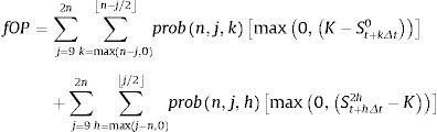
Substituting the striking price K into St+nΔtj we can obtain a fixed strike option as follow
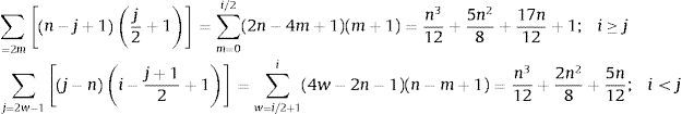
Finally we turn to the evaluation of the computational cost of the recursive algorithm for pricing maximum-minimum bidirectional options in trinomial CEV model. we determine the number of possible minima or maxima reached by the underlying asset at each node (i, j) (i=0,1,….,n; j=0,…….,2i) of the tree. Without loss of generality, we consider a trinomial tree with an even number, n, of time steps. We need distinguish two cases. The first considers the states of nature characterized by the triplet (i,j,k) and (i,j,h) such that i ≥ j, that I to say j=0,1,….,i. In Figure 1, we can easily observe that each node reached by a trajectory with j/2 up steps or i-j/2 up steps is characterized by j/2+1 minima or maxima for j=2m. and (j+1)/2 minima or maxima for j=2m+1 (m=0,1,….,i/2). Since in the tree there exist n−j+1 nodes characterized by j/2+1 and (j+1)/2 different minima or maxima. These nodes correspond to (n−j+1)*(j/2+1) and (n−j+1)*(j+1)/2 minima or maxima. The second case considers the states of nature characterized by the triplet (i,j,k) and (i,j,h) such that i<j i.e. j=i+1,….,2i, in the tree there exist j−n nodes characterized byn-j/2+1 and n-(j+1)/2+1different minima or maxima respectively for j=2w and j=2w-1(w=i/2+1,….,i). These nodes correspond to (j−n)*(n−j/2+1) and (j−n)*(n−(j+1)/2+1) minima or maxima. Thus the total number of minima or maxima in a trinomial tree with n time steps is equal to:
To compute the risk-neutral probability of each minimum or maximum in the tree, according to the forward induction procedure developed above, we have to implement two multiplications and one addition, hence, n3/6+7n2/4+22n/6 multiplications and n3/12+7n2/8+22n/12 additions (the node (0.0.0) has a risk-neutral probability equal to 1). Moreover, to the risk-neutral probability of each possible minimum price at the last time step, n, we have to associate the corresponding option payoff at maturity and then sum them up.
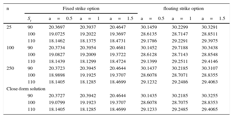
Table 1 illustrate the numerical results of the approach described above for evaluating floating strike and fixed strike maximum-minimum bidirectional options in the trinomial CEV model. The focus of the table is to check the approach performance and convergence. .in order to allow comparisons with other valuation methods, we choose the same option parameters as these used in Boyle and Tian (1999) illustrated in Duvydov and Linetsky (2001). The current asset price St may be 90 100 110, the time to maturity is T=6 months, the annualized risk-free interest rate r equals 10% and the volatility of the underlying asset rate of return is 25% per annum. The strike price is 100. The number of time steps n used ranges among 25, 100, 250. The elasticity factor a=0.5, 1 or 1.5. Furthermore, a close-form solution is computed with Davydov and Linetsky method expanded for comparison.
Valuation of the maximum-minimum bidirectional options in the trinomial CEV model.
| n | Fixed strike option | floating strike option | |||||
|---|---|---|---|---|---|---|---|
| St | a=0.5 | a=1 | a=1.5 | a=0.5 | a=1 | a=1.5 | |
| 25 | 90 | 20.3697 | 20.3937 | 20.4647 | 30.1459 | 30.2299 | 30.3291 |
| 100 | 19.0725 | 19.2022 | 19.3697 | 28.6135 | 28.7147 | 28.8511 | |
| 110 | 18.1462 | 18.1375 | 18.4731 | 29.1786 | 29.2291 | 29.3975 | |
| 100 | 90 | 20.3734 | 20.3954 | 20.4681 | 30.1452 | 29.7188 | 30.3438 |
| 100 | 19.0827 | 19.2009 | 19.3722 | 28.6128 | 28.7143 | 28.8548 | |
| 110 | 18.1439 | 18.1299 | 18.4724 | 29.1399 | 29.2511 | 29.4146 | |
| 250 | 90 | 20.3723 | 20.3945 | 20.4644 | 30.1437 | 30.2185 | 30.3107 |
| 100 | 18.9898 | 19.1925 | 19.3707 | 28.6078 | 28.7071 | 28.8355 | |
| 110 | 18.1405 | 18.1285 | 18.4699 | 29.1232 | 29.2486 | 29.4063 | |
| Close-form solution | |||||||
| 90 | 20.3727 | 20.3942 | 20.4644 | 30.1435 | 30.2185 | 30.3255 | |
| 100 | 19.0799 | 19.1923 | 19.3707 | 28.6078 | 28.7075 | 28.8353 | |
| 110 | 18.1405 | 18.1285 | 18.4699 | 29.1233 | 29.2485 | 29.4065 | |
Own elaboration.
As with other numerical method applications, prices from our trinomial CEV model is converge rapidly with all a value to the closed-form solution as the number of steps n increases. When n=25, on average, the value from our trinomial option pricing approach is closer to close-form solution than approximation solutions using other numerical method developed by Boyle, Tian and Bin. For n=100, the results show that the difference between the trinomial method and the closed-form solution is less than or equal to 0.01. The result with time step 250 is almost approach to close-form solution. The accuracy of results is similar to other numerical methods and the efficiency of recursive algorithm in the trinomial CEV model is higher than other numerical algorithm.
4ConclusionsA trinomial tree approximation for the CEV model was constructed to describe the evolution of the underlying asset with non-constant volatility. Once the trinomial tree has been built up, we proposed a recursive algorithm based on forward induction scheme to calculate transition probability of possible minimum or maximum reached by the underlying asset at each node over the trinomial tree when volatility varied with asset price level, further we use it to value different types of maximum-minimum bidirectional options. Numerical results show that the trinomial algorithm has satisfactory convergence and produces accurate prices for a wide range of parameter values of the CEV model compared with other numerical methods such as close-form solution method. In addition, for exotic path-dependent options that depend on the extreme of the process, the prices are quite sensitive to the specification of the process.
This paper is supported by National Natrual Foudation of China (NO: 71002098, NO: 61102009), Excellent Youth foundation of Beijing, China (YETP1652) and the Natural Sciences and Engineering Research Council of Canada (NSERC).
