


This work presents the development, assessment and comparison of four techniques for identifying dynamic parameters in an industrial redundant manipulator robot with 5 degrees of freedom. Based on the Lagrange–Euler formulation, a linear model of the robot with unknown parameters is obtained. Then, these parameters are identified using the following techniques: least squares, artificial Adaline neural networks, artificial Hopfield neural networks and extended Kalman filter. The parameters identified are validated by using them for computationally simulating the performance of the redundant manipulator robot, to which are imposed reference trajectories different from the ones used in the estimation. To relate the trajectories performed by the redundant manipulator robot with the estimated parameters, the following error indexes are calculated: Residual Mean Square, Residual Standard Deviation and Agreement Index. Finally, to determine the sensitivity of the model identified – due to the variations of the estimated parameters – a new simulation is conducted on the robot, considering that its parameters vary in a restricted range. In addition, the RMS error index of the trajectories performed is determined. After this step, the parameters of the redundant manipulator robot were successfully identified and, thus, its mathematical model was known.
Four closely related types of problem may be distinguished in the systems theory, namely modeling, analysis, estimation and control (Kessman, 2011). Modeling and estimation are extremely important to system identification. Modeling is a critical step when applying the systems theory to real processes aimed at obtaining a mathematical model that adequately describes a physical situation to be represented. To achieve this goal, several specifications should be considered, such as the limits and variables of the system. Then, the relationships between these variables need to be specified based on previous knowledge as well as on the assumptions about the uncertainties of the model, which characterize its structure. On the other hand, after obtaining an observable and identifiable model, the estimation of its unknown variables is addressed using an input/output dataset. Basically, there is a distinction between states and parameter estimation. Therefore, systems identification consists in experimentally determining a temporary behavior of a process or system, based on a mathematical model and using measured signals to determine such a behavior. The error (deviation) between the real process and its mathematical system has to be minimized to represent the real process or system in the best possible way (Isermann & Münchhof, 2011).
In the identification process, data characterizing the dynamics of the real process or system is first obtained. Then, a set of models is chosen and, finally, the best mathematical model of the set is selected. It should be noted that a mathematical model may be deficient due to reasons such as (Ljung, 1987):
- -
The failure in the numerical procedure conducted to find the best mathematical model, given a specific criterion.
- -
Ill-chosen criterion.
- -
No mathematical model satisfactorily describes the system.
- -
The information (data) is not sufficient for the selection of an appropriate mathematical model.
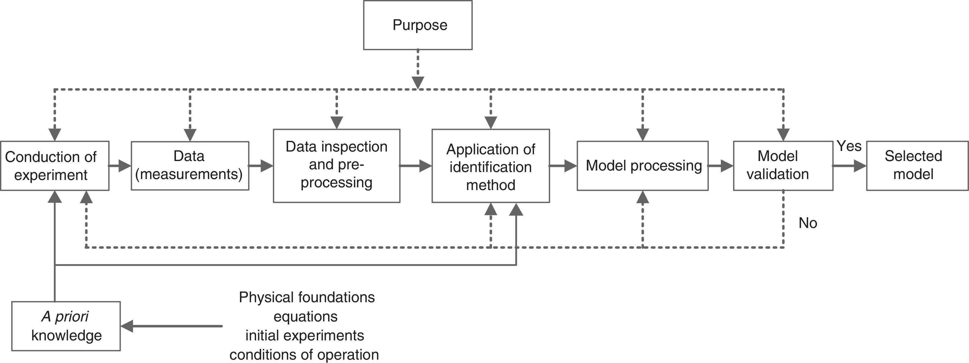
In summary, the general problem of systems identification may be expressed as: once known the structure and the value of some of the input and output variables of the system under study, it is necessary to determine the set of parameters that better adjusts to these measures (Anríquez, 2011). Figure 1 shows the general scheme of the identification of one system.
.")
System identification scheme (Isermann & Münchhof, 2011).
The methods for parameter identification applied to the redundant manipulator robot are explained below:
2.1Least squaresAmong the parameter estimation methods, least squares is widely used in the identification of manipulator robots (Bona & Curatella, 2005), since it is based on the use of a linear model inverse with respect to the parameters. This method allows estimating base inertial parameters from the measurement or estimation of torques and joint positions, optimizing the root mean square error of the model under the assumption that measurement errors are negligible. However, one problem in the application of this method is the noise sensitivity present in the measured data (Kessman, 2011), because noise will limit the accuracy of the obtained parameters as well as the convergence rate of the algorithm. To overcome this problem, it is suggested to generate excitation trajectories or to apply a filter to data (Ha, Ko, & Kwon, 1989).
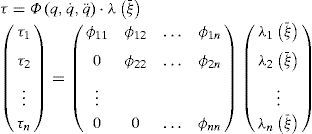
The dynamic model may be written as a set of unknown parameters linear equations, as shown in Eq. (1):
where τ corresponds to the generalized forces vector, q to the generalized coordinates vector, λ to the vector or unknown dynamic parameters and Φ to the observation matrix or regressor. By applying the identification model to the model shown in (1), the linear equation system in λ is obtained as:where ρ is the residual error vector. The estimated λˆ value may be obtained as:which is the same as calculating:2.2Adaline neural networks


A neural network consists of a set of simple processing units, which communicate by sending signals to one another through weighted connection. Adaline (adaptive linear element) is one type of neural network. For a one-layer network with one output and one linear activation function, the output is given by Eq. (5):

This network is able to represent a linear relation between the values of the output and input units. The purpose of this network is to produce a given value y=dp in the output when the set of values xip, i=0, 1, …, n. is applied to the inputs. It is intended to determine the coefficients (weights) wi, i=0, 1, …, n. so the input–output response is correct for a large number of arbitrarily chosen signal sets. In this case, the “delta rule” to adjust weights is used for Adaline, training the network in such a way that the best adjustment for each set of data composed of the input values xip and desired outputs dp is obtained. For each input datum, the network output differs from the desired value by dp−yp, where yp corresponds to the current output for this pattern. The “delta rule” uses a cost or error function based on this difference to adjust the weights. The error function is given by the mean squared error. Therefore, the total error E is defined by:
where the p index extends over the set of input patterns and Ep represents the error over the p pattern. This procedure allows for finding the value of all weights that minimize the error function by means of the gradient descent method:where γ is a constant of proportionality and, also:
Due to the linear relationship showed in (5):
and
Finally, we obtain:
where δp=dp−yp is the difference between the desired output and the current output for the p pattern.2.3Hopfield neural networksHopfield neural networks or HNNs can be used for estimating parameters on-line. In Hopfield's formulation, the dynamic of neuron i is described by the ordinary differential equation (12) (Alonso, Mendonça, & Rocha, 2009):
where ui is the neuron input i, fi is a strictly increasing, bounded, nonlinear continuous function, and Ci, Ri, Wij and Ii are parameters that correspond to a capacitance, a resistance, the weight associated to the connection of the j neuron with the i neuron, and the i neuron external input or bias. In Abe's formulation, it is assumed that Ci=1 and Ri=∞.
The considered system is linear with respect to the parameters, i.e. it has the form shown in Eq. (1), which (1) works under the following assumptions:
- (a)
τ, Φ∈C1.
- (b)
τ, Φ are bounded.
- (c)
τ(t), Φ(t) are known in each t instant.
- (d)
λ∈−c,cn for some c>0 unknown.
Given Abe's formulation, considering a network with N neurons, ui denotes the total input of the i neuron, its derivative with respect to time is:
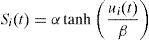
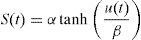
where Sj represents the state (or output) of the j neuron. The input-state relation for the i neuron is given by:where α, β>0 and, thus, ∀i∈N,t≥t0 Si(t)∈−α,α.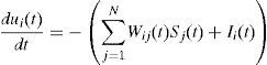
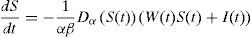
Using matrix notation, the network is as follows:
where S(t),I(t)∈ℝN×1 and W∈ℝN×N, under the state-space representation is:where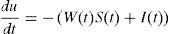
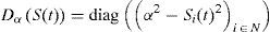
This a nonlinear and non-autonomous dynamic system whose architecture is completely determined by the N number of neurons, with characteristics given by α, β, W and I.
This work considers a HNN whose state S(t) over time t is taking as the estimation λˆ(t) of the λ parameter, in other words, λˆ(t)=S(t); implicitly, there is a network with as many neurons as parameters to estimate. Then, taking α=c, Eq. (14) guarantees that the trajectory generated for the network is in a feasible region of the estimation problem. Therefore, from the representation of states in Eq. (17), it is considered that: W=Φ(t)TΦ(t) and I=−Φ(t)Tτ. In this way, the dynamic of the HHN to be used as an on-line estimation algorithm is defined by:
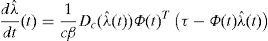
The advantage of using HNN to resolve the estimation problem is that inverting Φ(t)TΦ(t), is not necessary, since the latter might be ill-conditioned. In addition, given its structure, prior knowledge is not required for selecting λˆ(t0), i.e. of the initial estimation of λ.
Finally, the λ parameter is a globally, uniformly and asymptotically stable balance point of this HNN if the following sustains:
2.4Extended Kalman filter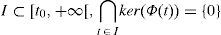
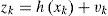
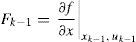
The extended Kalman filter is based on the direct dynamic model, which is nonlinear with respect to state and parameters. In this algorithm, physical parameters are considered under the use of an extended state. Kalman filter intends to estimate the x∈ℝn state of a process controlled in discrete time (Welch & Bishop, 2006). The algorithm has two steps that are executed in an iterative way, namely prediction, and correction or update of the state. However, when a system has non-linear characteristics, the formulation should be modified. This change in the algorithm is known as extended Kalman filter. In this case, the process will be represented by the following non-linear equations:
where f corresponds to a non-linear function that allows for knowing the relation between the previous step state vector k−1 and the u input with the current state vector k, according to the following procedure:
- 1.
Prediction stage
- 1.1
Prediction of the state:
- 1.2
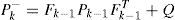
Prediction of error covariance matrix:
- 1.1
- 2.
Correction or updating stage
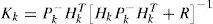
- 2.1
Kalman gain calculation
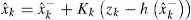
- 2.2
State update with measures Zk:
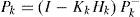
- 2.3
Covariance matrix update:
- 2.1

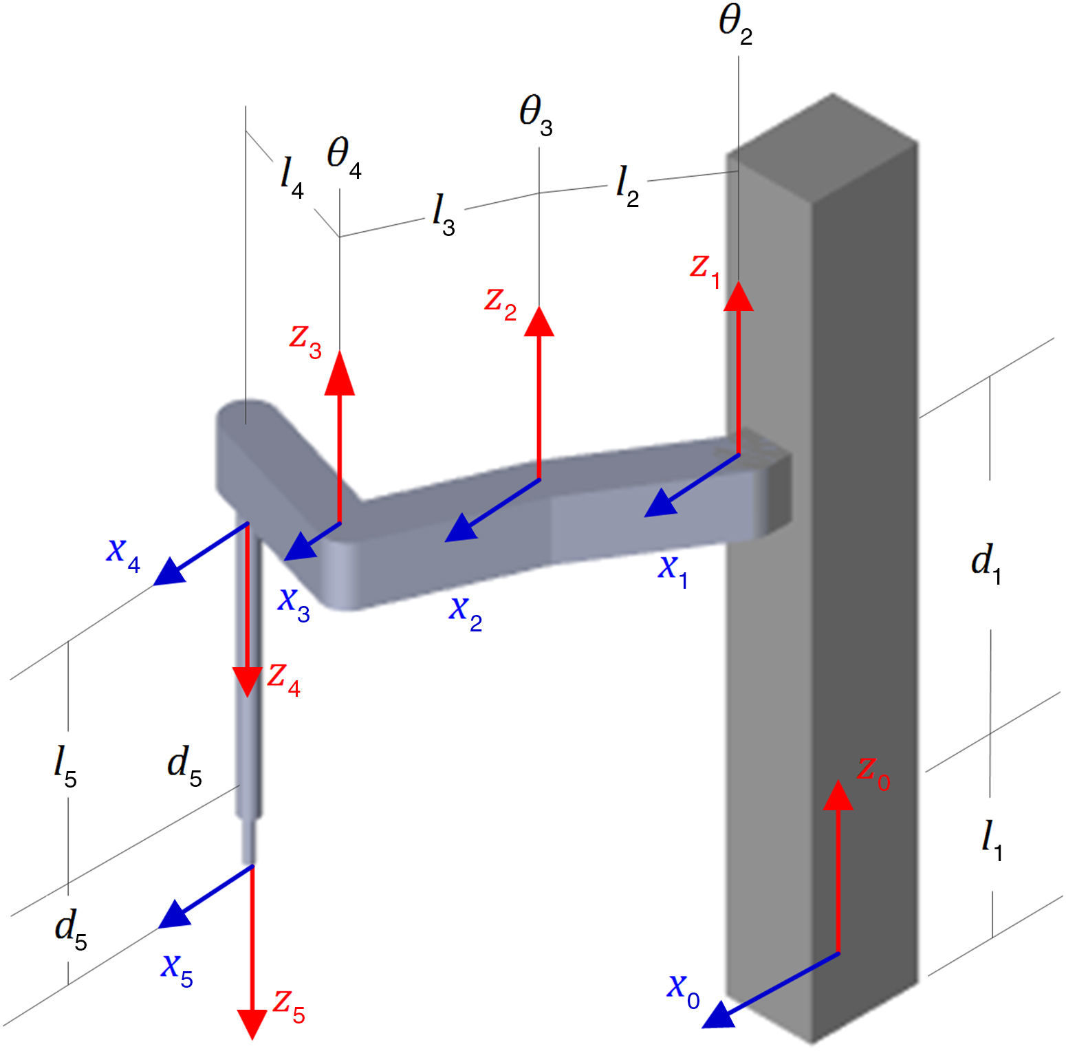
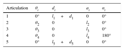
The manipulator robot used in this study is redundant, since it has five degrees of freedom (DOF), and a PRRRP configuration. Figure 2 shows a scheme of manipulator robot and its coordinate assignment. In addition, its Denavit–Hartenberg parameters are presented in Table 1.

The Lagrange–Euler formulation describes the behavior of a dynamic system in terms of work and energy stored in the system. The Lagrangian L is defined as:
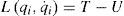
From this Lagrangian, the dynamic system equations of motion are given by:
where L is the Lagrangian function, T the kinetic energy, U the potential energy, qi the generalized coordinates, and Qi the generalized force applied to qi. The general form of a manipulator robot dynamic model is shown in Annex A.4Simulation of the methods for parameter identification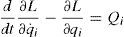
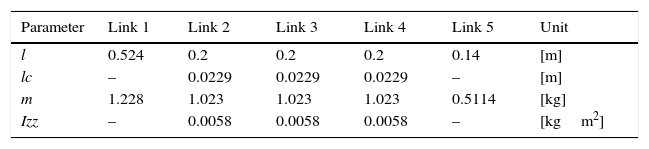
Table 2 shows the dynamic parameters of each link of the redundant manipulator robot (mass, length, center of mass and inertia) (Urrea & Kern, 2016).
In this work, we consider the following methods for identifying the parameters of the redundant manipulator robot: least squares, Adaline neural networks, Hopfield neural networks and extended Kalman filter. A brief description of these methods is presented below:
4.1Least squaresThe least squares procedure to estimate the parameters of each link of the redundant manipulator robot might be summarized in the following steps:
- -
Using some formulation, generate a robot model that is linear with respect to the inertial parameters.
- -
Reducing the inertial parameters to a set of base parameters.
- -
Determining the optimal trajectory of the parameters and optimize the excitation of the trajectories.
There is a number of methodologies to determine both the parameters influencing the systems dynamic and the set of minimum parameters required to identify the models of such systems (Choi, Yoon, Park, & Kim, 2011; Mayeda, Yoshida, & Ohashi, 1989; Mayeda, Yoshida, & Osuka, 1990; Radkhah, Kulic, & Croft, 2007). This work considers a numerical method that allows for identifying the set of independent parameters of the redundant manipulator robot, based on the analysis of the kernel of the regressor.
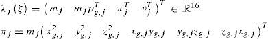
For a redundant manipulator robot with j links, ten inertial parameters are considered per link:
where mj,pg,j=xg,jyg,jzg,jT and vj=Ixx,jIyy,jIzz,jIxy,jIxz,jIyz,jT are the mass, the position of the center of gravity, and the vector with the elements of the inertia tensor of the j link, respectively. A linear form may be composed by grouping the parameters as follows:where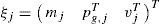
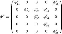
The regressor Φ is not always linearly independent or has a full rank, thus there might not be a unique solution. Nevertheless, it is possible to reduce the number of unknown parameters and transform the system into: τ=Φ*·λ*, where λ* is the vector for regrouped parameters. It is hard to find the linear relation between dependent and independent columns of the regressor, since dynamic relationships are complex. To find this relation, the kernel of the matrix is used, which denotes the relation between columns dependent and independent from the regressor in linear combinations. In this way, the new grouped parameters λ* and the full rank matrix Φ* may be found. The calculation is conducted in a recursive way, starting from the n joint up to the articulation 1.
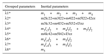
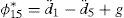
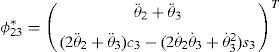
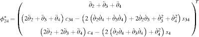
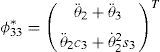
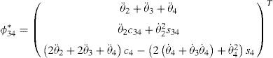
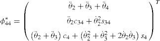
In this case, the vector of regrouped parameters λ* is composed of eight elements to be identified, which are presented in Table 3. The structure of the regressor Φ*∈ℝ5×8 is described in Annex B.
When a system identification experiment is designed, it is necessary to consider a trajectory that sufficiently excites the redundant manipulator robot parameters during the movement. Otherwise, some parameters will be impossible to identify, or will become too sensitive to noise (Swevers, Ganseman, De Schutter, & Van Brussel, 1996). Meanwhile, since the regressor Φ* depends on joint coordinates and its time derivatives, when the manipulator robot executes a particular trajectory GDL·npts equations will be obtained, generating an over-determined system. Thus, considering the points traveled in the trajectory, the system is given by the expression:
where τ is the torque/force vector ∈ℝGDL⋅npts,W is the ∈ℝGDL⋅npts×np system observation matrix, λ* is the vector of the grouped parameters ∈ℝnp,nptos is the number of samples and np corresponds to the number of parameters grouped. Then, to identify the parameters it is necessary to calculate:
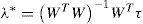
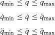
Parameters accuracy is closely related to the observation matrix W, so the purpose is to obtain a well-conditioned matrix that allows for enhancing the estimation results (Wu, Wang, & You, 2010). This implies finding the denominated “excitation trajectories”, which correspond to an optimization problem that consists in minimizing a function like the one presented in (37) subjected to the constraints of Eq. (38):
where function f satisfies the criterion kW=(σmax/σmin),q,q˙,q¨ are the generalized coordinates of position, velocity and acceleration, respectively, σmax is the highest singular value of W and σmin the lowest singular value of W.4.1.2Trajectory parameterization
The prismatic joints motion does not participate in the rotary joint dynamics. Thus, without loss of generality, trajectory optimization is only applied to rotary joints, since they are in conflict with the parameter estimation of least squares. The reverse is true for the prismatic link with linear characteristics. The excitation trajectories are planned using a polynomial of degree five (Benimeli, 2005) in the form of Eq. (39) and the elements to be optimized are their coefficients: a0i, a1i, …, a5i:

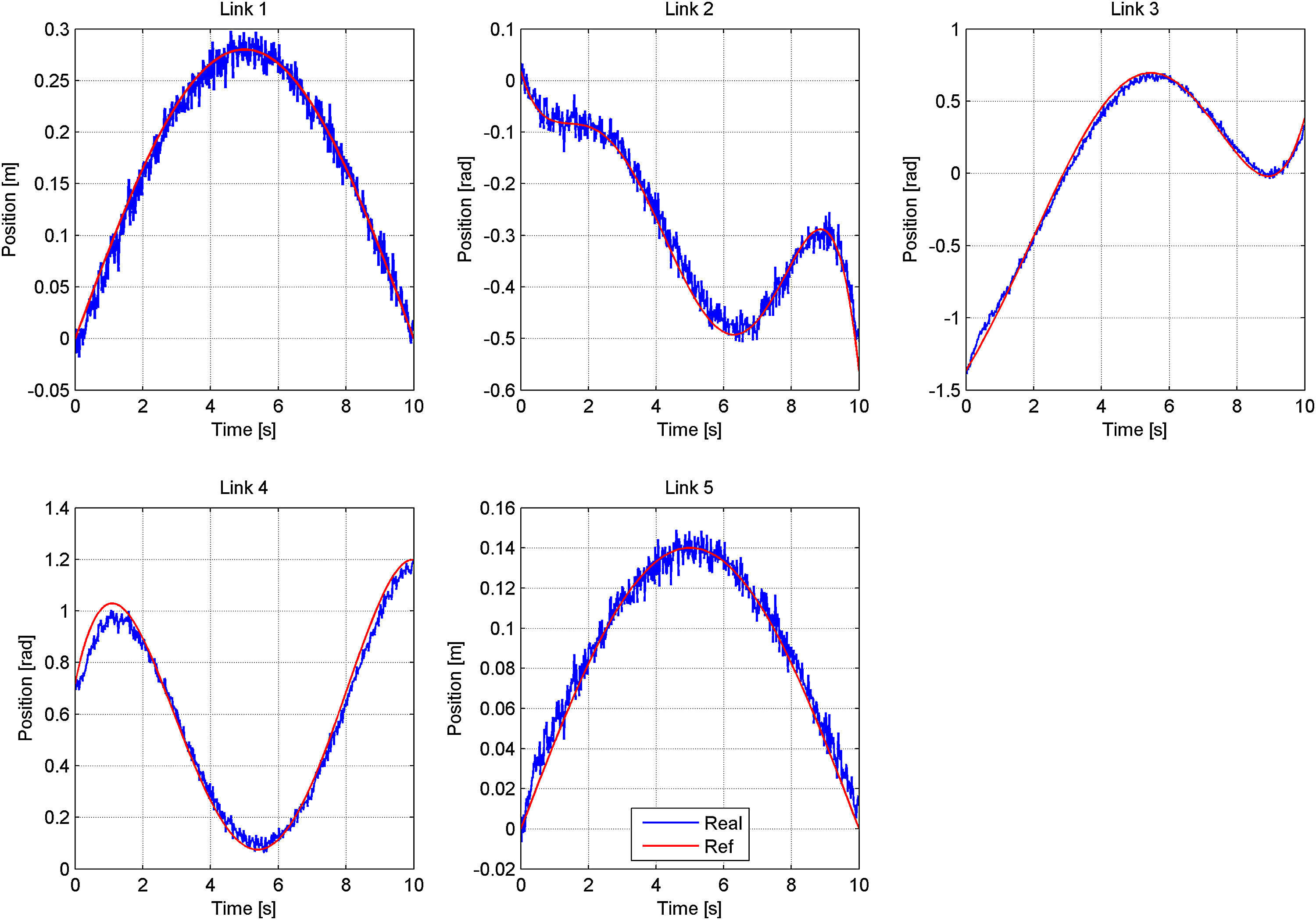
Reference sinusoidal trajectories are applied to the first and fifth link (prismatic joints). All the reference and output trajectories of all the joints of the redundant manipulator robot are shown in Figure 3. An electronic noise is observed due to the sensing (measuring) of the output trajectories.
4.2Adaline neural networks
Applying the linear model formulation to the parameters τ=Φ*·λ* (see Annex B), we have that:
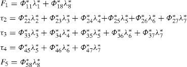
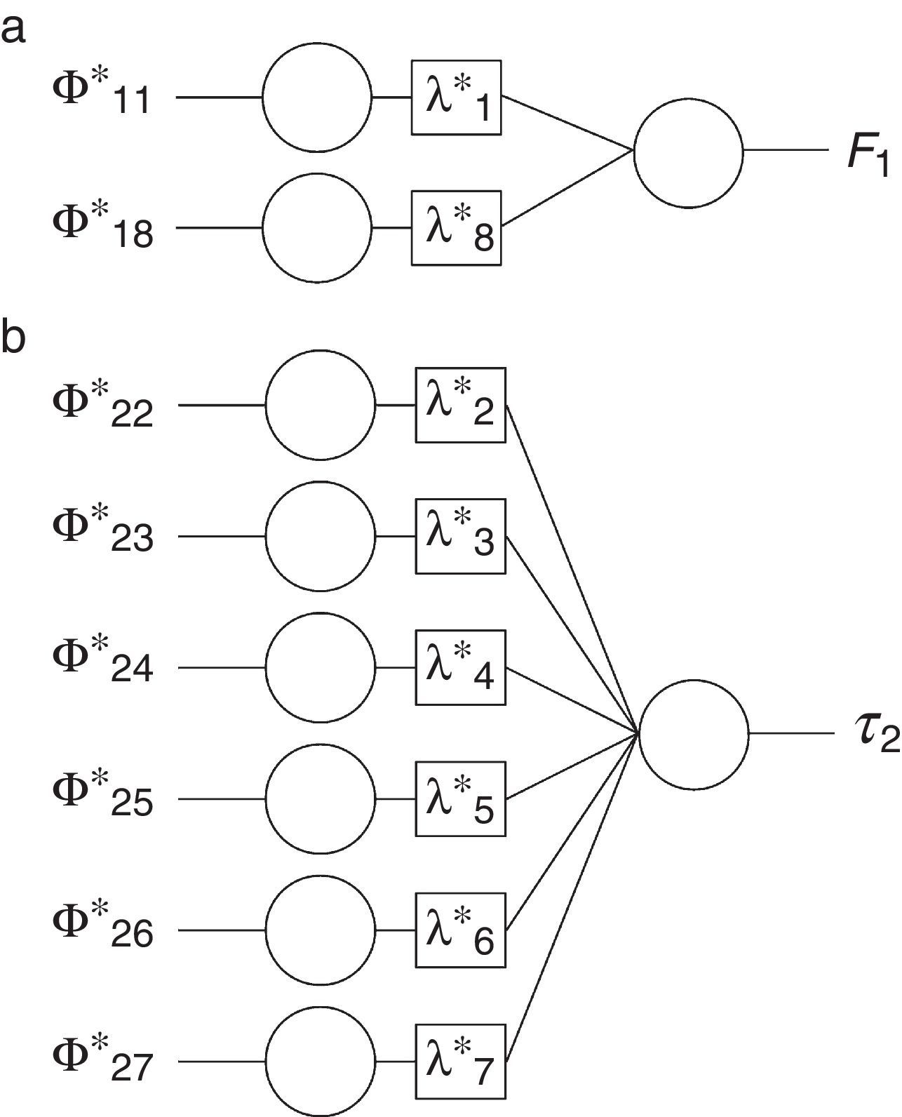
Therefore, when using an Adaline network, the parameters to be identified coincide with the network weights. Below, one-layer neural networks are designed with their inputs corresponding to the elements of the regressor and their outputs to the elements of torque/forces. Figure 4 shows the scheme of the networks used for the identification of the parameters of the redundant manipulator robot.
4.3Hopfield neural networks Network 1. (b) Network 2.")
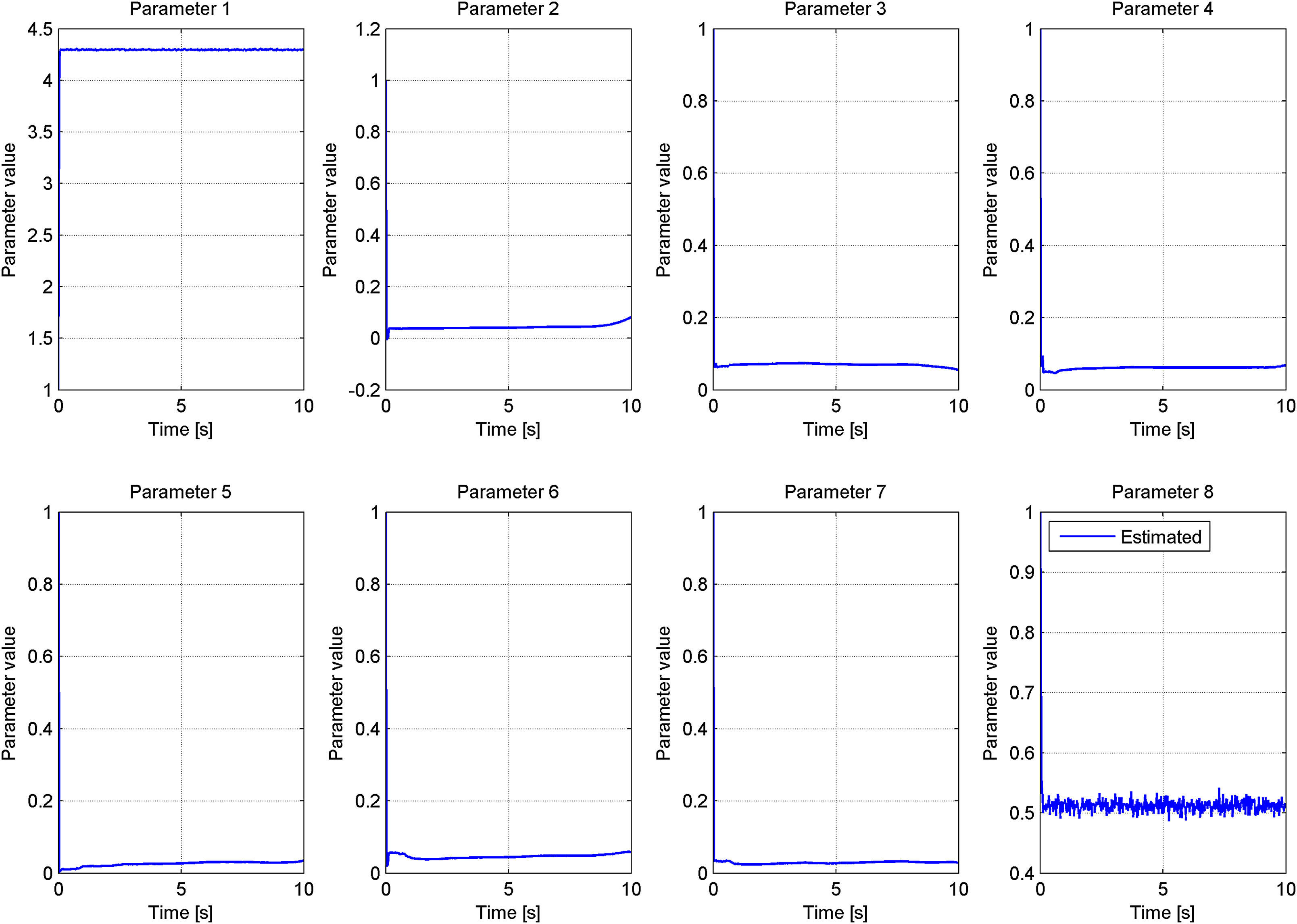
For satisfactorily identifying the parameters of the redundant manipulator robot, all intervals of t⊂0, +∞ should satisfy the condition given by Eq. (20). Figure 5 shows the response produced by the HNN. The last estimated valued is used for the comparison.
4.4Extended Kalman filter
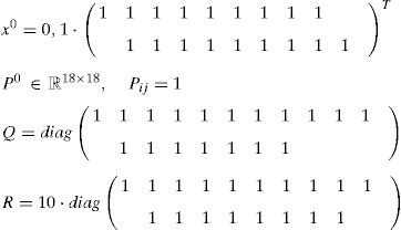
In this method, use is made of the dynamic model of the redundant manipulator robot, i.e. the joint coordinates that mathematically depended on the force/torque applied to them are used. The direct dynamic model is symbolically calculated from the Lagrange–Euler formulation and the grouped parameters described in Table 3, and then is expressed in the state variables presented in Eq. (41). The parameters to be identified are included in an extended state of the algorithm with a time derivative of null values, as shown in Eq. (42):
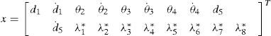
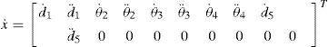
Euler approximation is used for the equations whose time derivative was calculated, as seen in Eq. (43):
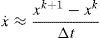
Therefore, from the equation above, xk+1=xk+Δt⋅x˙k is obtained, whose sampling time is Δt=0.02. In turn, the initial state vectors used are initial error covariance matrix, process noise covariance matrix and observation covariance matrix, as presented in Eq. (44):
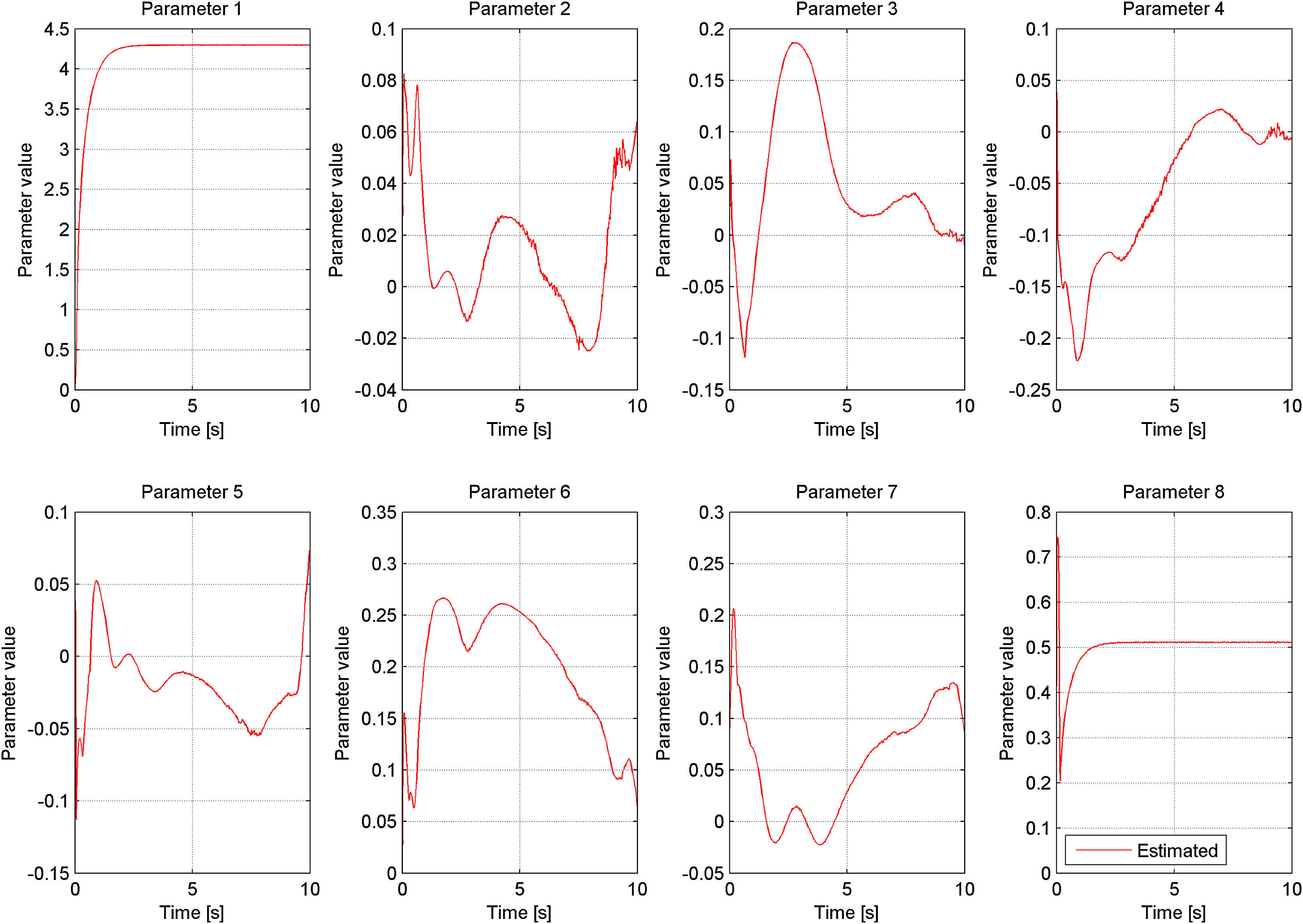
The reference trajectories used in this identification process are the same applied to the least square methods, i.e. those presented in Figure 3. The evolution of the parameter estimation curves is shown in Figure 6. In this case, the last value of the estimation is considered for error comparison.
5Results
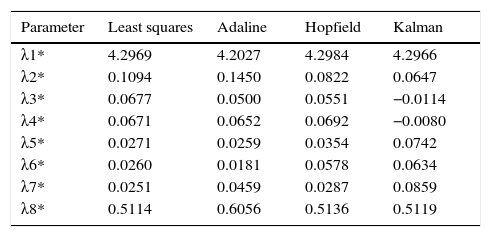
Table 4 shows the base parameters identified for each of the studied methods.
Estimated parameters.
| Parameter | Least squares | Adaline | Hopfield | Kalman |
|---|---|---|---|---|
| λ1* | 4.2969 | 4.2027 | 4.2984 | 4.2966 |
| λ2* | 0.1094 | 0.1450 | 0.0822 | 0.0647 |
| λ3* | 0.0677 | 0.0500 | 0.0551 | −0.0114 |
| λ4* | 0.0671 | 0.0652 | 0.0692 | −0.0080 |
| λ5* | 0.0271 | 0.0259 | 0.0354 | 0.0742 |
| λ6* | 0.0260 | 0.0181 | 0.0578 | 0.0634 |
| λ7* | 0.0251 | 0.0459 | 0.0287 | 0.0859 |
| λ8* | 0.5114 | 0.6056 | 0.5136 | 0.5119 |
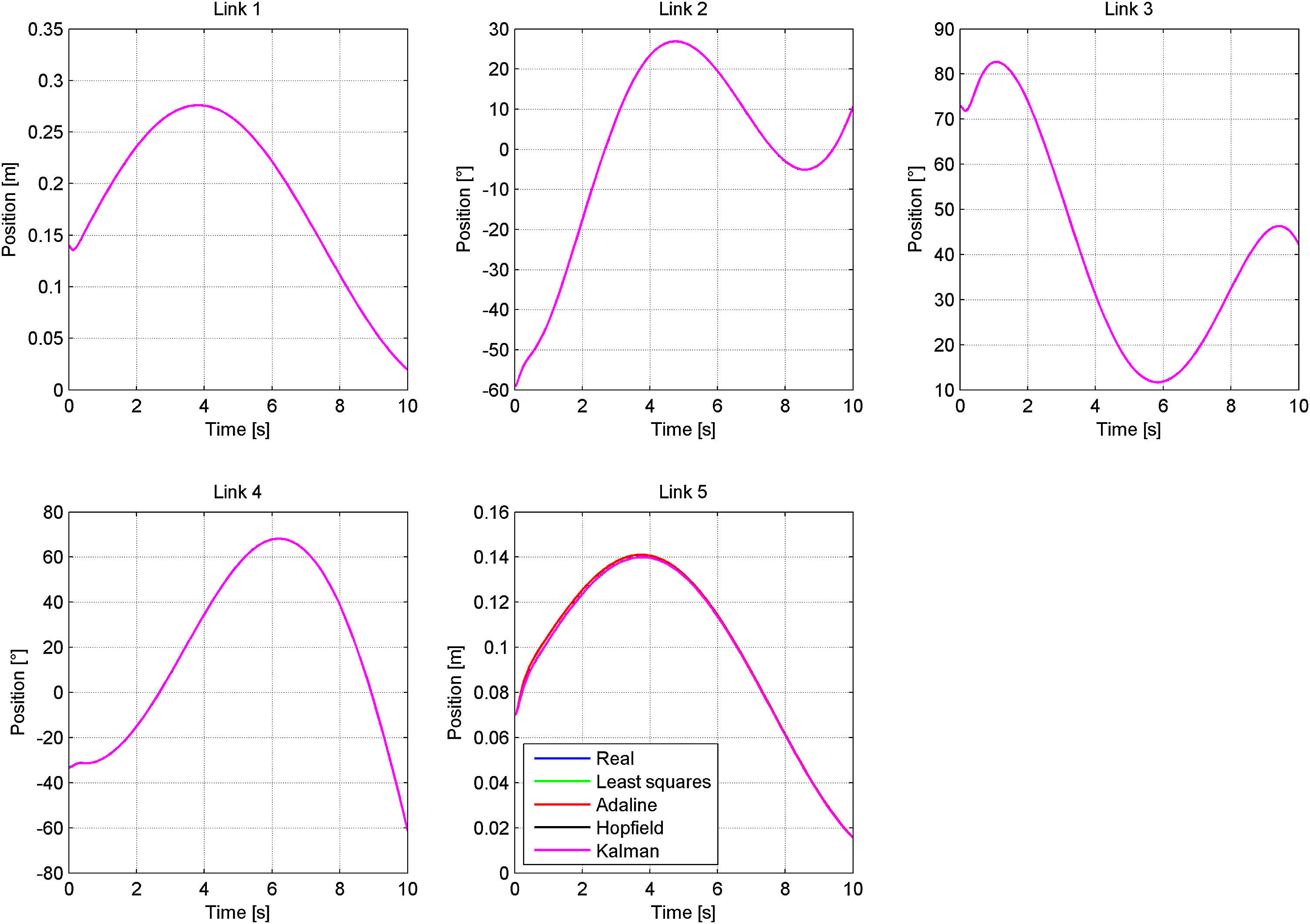
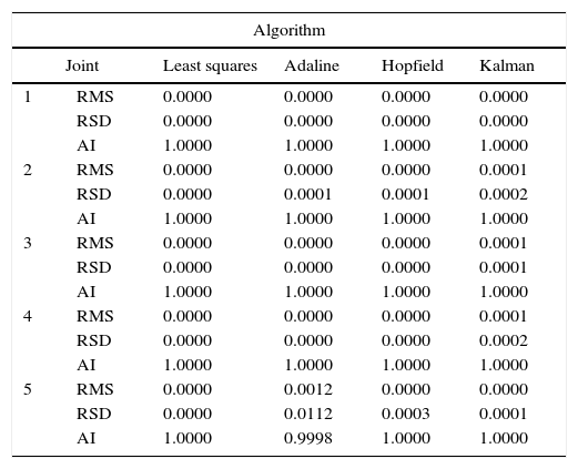
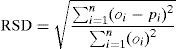
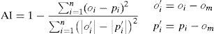
To validate the identified parameters, they are used in performance simulations on the redundant manipulator robot. In these simulations, validation trajectories different from those used in the estimation are imposed to the robot. To relate the trajectories performed by the redundant manipulator robot with the estimated parameters of the same, the following error indexes are calculated: Residual Mean Square (RMS), Residual Standard Deviation (RSD) and Agreement Index (AI); which are mathematically represented in Eqs. (45)–(47), respectively. RMS and RSD correspond to normalized percentage values between 0 and 1; indexes that explain the dispersion and deviation of the series, respectively. In addition, the AI index indicates the trend of the two series to be compared; the values that adopts may fluctuate between 0 and 1, where: 1 corresponds to a perfect match and 0 to absence of agreement. The trajectories performed by the redundant manipulator robot are shown in Figure 7, and their error indexes in Table 5. It should be noted that the trajectories presented in Figure 7 are basically overlapped, and that the values of the parameters do not show high sensitivity to following imposed trajectories:
where oi are the values observed, om the mean value of the observations, pi are the predicted values and n is the total number of observations.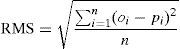

Error indexes.
| Algorithm | |||||
|---|---|---|---|---|---|
| Joint | Least squares | Adaline | Hopfield | Kalman | |
| 1 | RMS | 0.0000 | 0.0000 | 0.0000 | 0.0000 |
| RSD | 0.0000 | 0.0000 | 0.0000 | 0.0000 | |
| AI | 1.0000 | 1.0000 | 1.0000 | 1.0000 | |
| 2 | RMS | 0.0000 | 0.0000 | 0.0000 | 0.0001 |
| RSD | 0.0000 | 0.0001 | 0.0001 | 0.0002 | |
| AI | 1.0000 | 1.0000 | 1.0000 | 1.0000 | |
| 3 | RMS | 0.0000 | 0.0000 | 0.0000 | 0.0001 |
| RSD | 0.0000 | 0.0000 | 0.0000 | 0.0001 | |
| AI | 1.0000 | 1.0000 | 1.0000 | 1.0000 | |
| 4 | RMS | 0.0000 | 0.0000 | 0.0000 | 0.0001 |
| RSD | 0.0000 | 0.0000 | 0.0000 | 0.0002 | |
| AI | 1.0000 | 1.0000 | 1.0000 | 1.0000 | |
| 5 | RMS | 0.0000 | 0.0012 | 0.0000 | 0.0000 |
| RSD | 0.0000 | 0.0112 | 0.0003 | 0.0001 | |
| AI | 1.0000 | 0.9998 | 1.0000 | 1.0000 | |
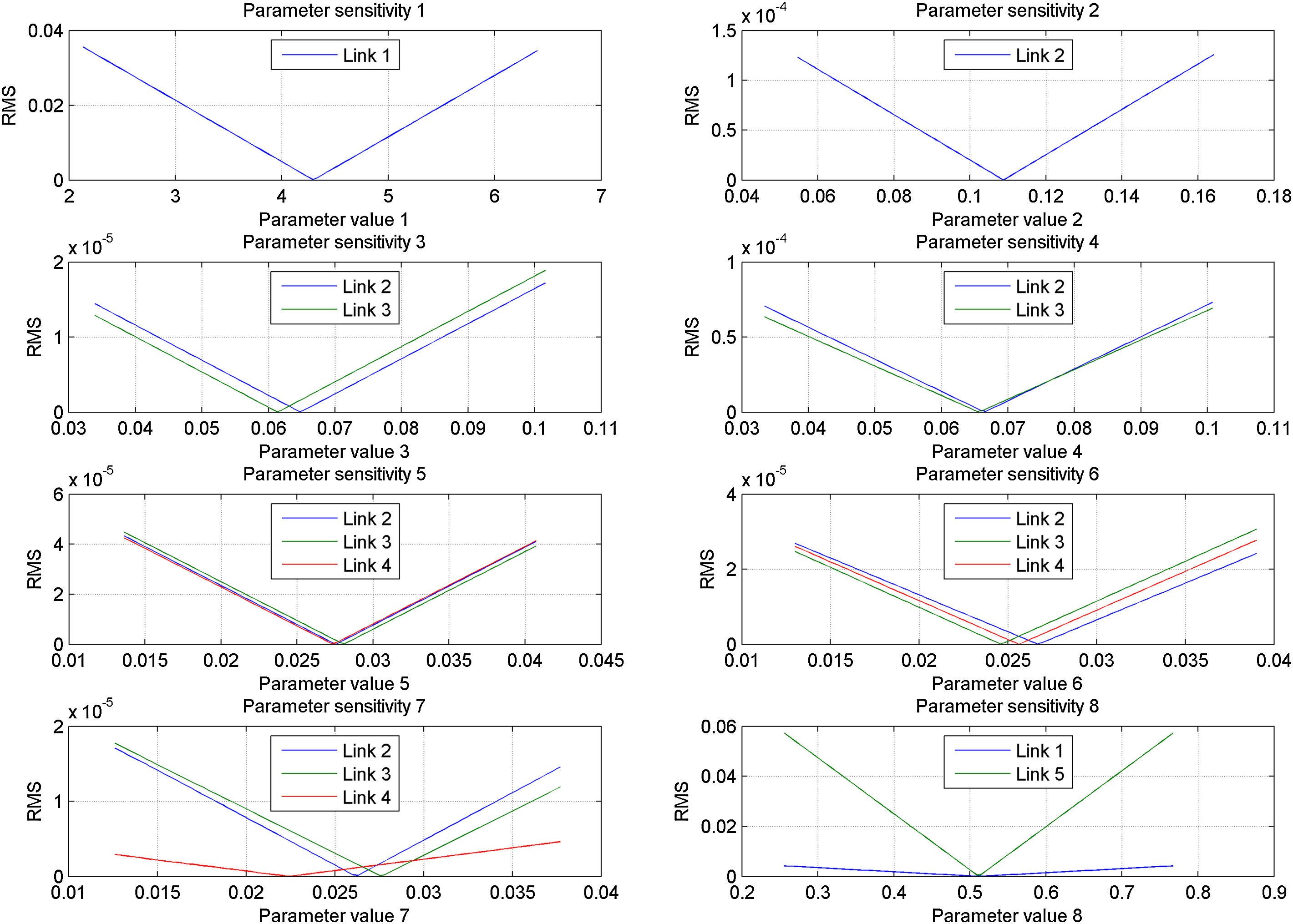
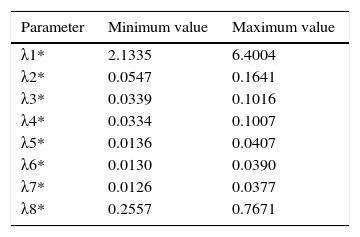
To determine the sensitivity of the identified model, due to the variations of the estimated parameters, the redundant manipulator robot is simulated, considering that its parameters varied in a restricted range of values. Also, its RMS error index is calculated between the trajectories described. Table 6 presents the range of values for the variations in the ±50% parameters. In Figure 8, the evolution of the RMS index of the performed trajectories, with respect to each estimated parameter, is illustrated.

In this paper, we presented the identification of the parameters of an industrial redundant robot with 5 DOF. By means of the Lagrange–Euler formulation, the linear model with unknown parameters was obtained. To identify these parameters, four methods were used, assessed and compared, namely least squares, Adaline neural networks, Hopfield neural networks, and extended Kalman filter.
The identified parameters were validated by computationally simulating the performance of the redundant manipulator robot. To this end, reference trajectories different from those used in the estimation were imposed to the robot.
To relate the trajectories described by the redundant manipulator robot with its estimated parameters, the following error indexes were calculated: Residual Mean Square, Residual Standard Deviation and Agreement Index.
The sensitivity of the identified model to parameter variation is low.
The parameters of the redundant manipulator robot were successfully identified and, therefore, the robot mathematical model was known. Thanks to this achievement, it is now possible to design, simulate, compare, validate and implement diverse strategies for controlling this industrial redundant robot with 5 DOF.
Conflict of interestThe authors have no conflicts of interest to declare.
This work was supported by Proyectos Basales and the Vicerrectoría de Investigación, Desarrollo e Innovación of the Universidad de Santiago de Chile, Chile.
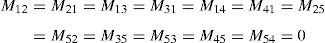
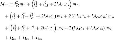
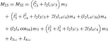
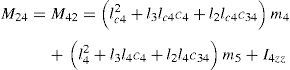
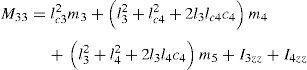
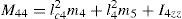
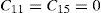
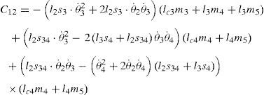
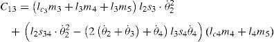
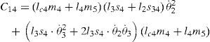
The dynamic model of the manipulator robot was developed in (Urrea & Kern, 2016). Below are presented the components of the inertia matrix, the centrifugal force and Coriolis force vector and the gravity vector, respectively.
where s3=sinθ3, s4=sinθ4, c3=cosθ3, c4=cosθ4, s34=sin(θ3+θ4) and c34=cos(θ3+θ4); m1, m2, m3, m4, m5 and l1, l2, l3, l4, l5 represent the masses and length of the first, second, third, fourth and fifth link, respectively; lc2lc3 and lc4 express the lengths from the origin to the mass center of the second, third and fourth link, accordingly. Finally, l2zz, l3zz and l4zz represent the moments of inertia of the second, third and fourth links, referred to the z axis of each joint, respectively.


Peer Review under the responsibility of Universidad Nacional Autónoma de México.