


In this paper, a fractional differential zero phase (FDZP) 2D filter is constructed which is based on the technique of zero-phase filtering utilizing the concept of R–L integral with fractional differentiation. The constructed filter mask is used to denoise an image with the forward-backward processing which gives high robustness for images corrupted with Gaussian noise with varying degree of standard deviation and with speckle noise. The proposed FDZP 2D filter has high edge preserving capability that is also quantitatively evaluated using the peak signal-to-noise ratio (PSNR) performance measure. From the quantitative analysis, the PSNR value is much better than those obtained using Gaussian smoothing, Alexander fractional differential (AFD), Alexander fractional integral (AFI), anisotropic diffusion and kuan filters for standard and ultrasonic image of liver, respectively. The experiments illustrate that the improvements achieved are compatible with other existing filters.
One of the fundamental challenges in image processing and computer vision is image denoising. Noise is a random signal that corrupts an image at the time of image acquisition. Efficient methods for the recovery of the original image from the noisy image are extensively explored in the literature (Grieg, Kubler, Kikinis, & Jolesz, 1992; Motwani, Gadiya, Motwani, & Harris, 2004). There are two types of models for image denoising, namely, linear and non-linear. The linear models, such as Gaussian and wiener filters, work well in reducing the noise present in flat regions of the images but they are incapable of preserving image texture and the edge information. Such limitation is removed using the non-linear models that have better edge preserving capability than linear models. The fractional calculus has been applied by numerous researchers in various fields (Kilbas, Srivastava, & Trujillo, 2006; Podlubny, 1998) related to image texture enhancement (Gao, Zhou, Zheng, & Lang, 2011; Hu, Pu, & Zhou 2011b) and Jalab and Ibrahim (2012) and image denoising (Cuesta, Kirane, & Malik, 2012; Das, 2011; Hu, Pu, & Zhou, 2011a; Miller & Ross, 1993). The results, which were computed using these operators, showed high robustness against different types of noise (Artal-Bartolo, 1994; Das, 2011) implemented a fractional integral filter using fractional integral mask windows on eight directions based on Riemann–Liouville definition of fractional calculus. The efficiency of the method was evaluated by computing the PSNR=27.35 at Gaussian noise with a standard deviation σ=25 for the boat image. Hu, Pu, and Zhou (2011b) proposed an algorithm that is a based on fractional calculus definition of Grünwald–Letnikov (G–L) using fractional integral mask windows. G–L achieved fine-tuning, by setting a smaller fractional order, and controlled the effect of image denoising by iteration. Jalab and Ibrahim (2015) proposed two image denoising filters AFD & AFI using the concept of alexander polynomial with fractional calculus. The efficiency of the proposed filters was evaluated by computing average PSNR=26.47, 27.01, respectively, for Gaussian noise with σ=25 for the cameraman image. Wang, Pan, Gao, and Zhuang (2014) proposed a fractional zero phase filters for ECG signal denoising that gives better results when compared to other existing filters in the literature. In this paper, the ECG filtering technique is extended further from 1D to 2D with the utilization of fractional differentiation to denoise an image.
This paper is organized as follows: Section 2 presents the overall framework of our proposed FDZP 2D filter in which the mathematical analysis is described. In Section 3, the construction of the FDZP 2D filter and the procedure of denoising of an image are presented. The simulation results and the comparison with other methods are explained in Section 4, respectively. Finally, in Section 5 the conclusion is presented.
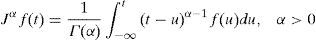
2Mathematical background2.1Fractional order RL integral filterFor a one-dimensional signal, the definition of filter is obtained from the generalized definition of integer integral filter. From the cauchy integral formula which states that if f(t) is an analytic function in a complex plane, the formula Das (2011) is:
where N is the set of positive integers and extended from n∈N to real number (α>0). This methodology is used to define the RL approach. In this approach, the identity operator is defined as J0 i.e., J0=1, and a, the orderd integral operator, is written as Ja and also assumes the lower limit of cauchy integral formula is set to zero (a=0). According to these assumptions, we define the definition of the a-order RL fractional integral from (1) as:where the f(t) signal has a duration from [0,t] and Γ(.) is the gamma function.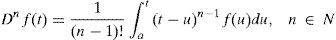
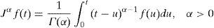
If we assume that the f(t) signal is causal then Eq. (2) is written as:
After analyzing Eq. (3), the kernel function for the Ja operator is defined as:
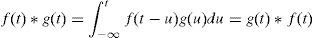
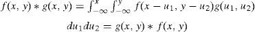
But we know the convolution of the casual signals are defined as:3Proposed 2-dimentional zero phase filter3.1Proposed mathematical background for 2D filter design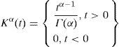
The definition of R–L filter for 2D is basically a generalized case of 1D. In 2D, the cauchy integral formula is stated as if f(u1) and f(u2) are analytic functions in a complex plane, then the formula is written as:
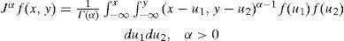
where N is the set of positive integers and extended from n∈N to real number (a>0). This same methodology is used to define the RL approach. The generalized formula of a-order RL fractional integral in 2D (5) is written as:where f(u1) and f(u2) are the variation of pixels of images along x and y directions, respectively, having a duration of [0,T], and Γ(.) is the gamma function.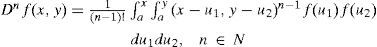
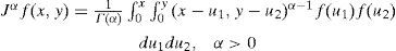
If we assume that the f(u1) and f(u2) functions of the image along x and y directions are causal, then Eq. (6) is written as:
From using Eq. (7), the kernel function is written as:
Here, r is the location of the pixels in the mask. The value of r is nothing but the location of pixel if the value along x and y direction are equal, i.e., with the help of kernel equation we have easily obtained the diagonal pixel values. But the definition of the convolution of the image functions are defined as:From the comparison of Eqs. (7) and (9), the obtained equation is written as:At last from the above definition of the kernel, the 2D mask is constructed which is used to denoise an image.3.2Construction of FDZP filter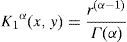

The filter mask which is constructed using the proposed mathematical background is differentiated along the x and y direction to obtained satisfactory results. Hence, the modified filter equation is written as:
were μ is the fractional differential order and (x, y) are the location of pixel in the constructed mask.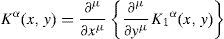
On solving Eqs. (8) and (10), the simplified equation of mask is written as
From Eq. (11), we conclude that the diagonal elements of mask are easily obtained. Here the values of r are 1, 2, 3, 4, …, N, respectively. Where N is the location of the diagonal element in the constructed mask. With increasing the mask size above 3×3, the complexity of the algorithm increases and the PSNR value decreases. To reduce the complexity, computational time and achieve desirable PSNR the size of mask should be 3×3. The values of the diagonal elements are easily obtained by setting r=1, 2, 3 for 3×3 mask and other pixel values must be taken as zero. By using this mask we obtain the weighted pixel values of mask in each direction, i.e., 180°, 0°, 90°, 270°, 135°, 315°, 45°and225° are the same. Hence, this mask is rotation invariant. The proposed constructed kernel in Figure 1 is obtained using the combination of the kernels in each direction.3.3Fractional forward-backward processing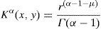

After the construction of filter, the concept of fractional forward-backward filtering is used to denoise an image with the use of the constructed FDZP filter proposed. The procedure for denoising of an image is shown in Figure 2.

The detailed description of the fractional forward-backward filtering is explained as follows: suppose that an image I(x, y), x, y∈0,T where the maximum possible pixel value is 255, is corrupted by additive white Gaussian noise. First, the corrupted image I (x, y) is fed on the constructed fractional 2D filter Kα(x, y) and the output image is obtained as yf(x, y). Second, yf(x, y) is reversed to produce the reverse image, i.e. yfR(x, y)=yf(T−x, T−y). Third, yfR(x, y) is again fed into the fractional 2D filter Kα(x, y) and the output image is obtained as yfbR(x, y). Finally, yfbR(x, y) is reversed again to get yfb(x, y). Analytically, it can be shown that the last obtained image output yfb(x, y) is not phase distorted as the output image which is highly suppressing the noise from the corrupted image. The above procedure can be represented mathematically as follows:
where Kα(x, y) is the kernel function of the fractional 2D filter.4Results and discussion4.1Image database and performance measures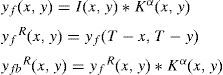

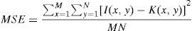
The experiments were performed on MATLAB 7.12.0 (R2011a) with the Windows platform. The proposed filtering mask was tested on the standard images taken from Rafael Gonzalez and Woods (2002), medical test image database available at (http://decsai.ugr.es/∼javier/denoise/testimages accessed on May, 2014), which contain grayscale, color and ultrasonic images of the liver. The performance of the proposed FDZP 2D filter was evaluated by computing PSNR. It is defined in terms MSE and is related inversely proportional to MSE, “the average of the squared error between the two images is called mean square error (MSE)”. A higher value of PSNR means that the denoised image is of a good quality. The PSNR measures in decibels and is formulated as Eq. (13):
where I(x, y), K(x, y) are denoted as the original and denoised images, respectively.4.1.1Selection of mask size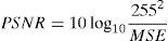
The mask size also plays an important role in denoising an image. On experimenting with the different mask sizes, i.e., from 3×3, 5×5, 7×7, … for a lena image corrupted by Gaussian noise of σ=25, it is observed that the maximum PSNR value decreases. For example: using 3×3 mask it was 34.36 and when 5×5 was used the maximum PSNR was reduced to 30.02. Hence, the mask size equal to 3×3 is chosen.
4.1.2Choice of fractional parametersIn FDZP 2D filter, the denoising capability is controlled by two main parameters, i.e., μ and α. The values of these parameters are chosen so as to achieve maximum PSNR. When the standard images i.e., Lena, Cameraman, Baboon, House are corrupted with Gaussian noise of σ=25. The maximum PSNR is obtained for the values of parameters μ, α equal to 0.21, 0.95, respectively. To select the values other than μ=0.21, α=0.95 the PSNR value is reduced. It is clearly shown in Figures 3 and 4.
4.2Visual perception

For the human visual perception, we perform the two sets of experiments by adding different noises to the original images.
4.2.1Addition of Gaussian noiseIn this set of experiments, artificial Gaussian noise with different standard deviations equal to 15, 20, and 25 were added to the Lena, Cameraman, House and Baboon images. The corrupted image is then filtered using Gaussian, AFI, AFD and the proposed FDZP 2D filter. For the sake of visual comparison with the existing techniques, only those images are shown for which the results were available at a particular standard deviation value. The results for the grayscale lena image corrupted with the Gaussian noise with standard deviation equal to 15 can be visualized in Figure 5. Figure 5(a) shows the original image, Figure 5(b) shows the corrupted image or noisy image, Figure 5(c–f) shows the image filtered using Gaussian smoothing, AFD, AFI and the proposed FDZP 2D filters. From the analysis, it can be concluded that the proposed approach efficiently denoises the corrupted image.
 Original image, (b) image with Gaussian noise, σ=15, (c) Gaussian smoothing filter, (d) AFD filter, (e) AFI filter, (f) proposed FDZP 2D filter.")
Robustness of the designed FDZP 2D filter at higher values of standard deviation can be visualized in Figure 6. Figure 6(a) shows the original color baboon image, Figure 6(b) shows the noisy image in which Gaussian noise with a standard deviation σ=20 is added, Figure 6(c–f) shows the filtering results obtained using Gaussian smoothing, AFD, AFI and the proposed FDZP 2D filters. From this analysis it can be concluded that the proposed approach efficiently denoise the corrupted image.
 original image, (b) image with Gaussian noise σ=20, (c) Gaussian smoothing filter, (d) AFD filter, (e) AFI filter, (f) Proposed FDZP 2D filter.")
Further, when the standard deviation of corrupted image is increases to σ=25 then the noise is highly affect the original image but our proposed FDZP filter gives much better denoised image as compared with existing approaches. The robustness of the proposed FDZP 2D filter at higher values of standard deviation can be visualized in Figure 7. Figure 7(a) shows the original grayscale cameraman image, Figure 7(b) shows the noisy image in which Gaussian noise with standard deviation σ=25 is added, Figure 7(c–f) shows the filtering results obtained using Gaussian smoothing, AFD, AFI and proposed FDZP 2D filters. From all the analysis it can be concluded that the proposed approach efficiently denoises the corrupted image.
 original image, (b) image with Gaussian noise σ=25, (c) Gaussian smoothing filter, (d) AFD filter. (e) AFI filter, (f) proposed FDZP 2D filter.")
Similar conclusions were drawn when the experiments were done on the colored house image with the same value of standard deviation as shown in Figure 8(a–f).
 original image, (b) image with Gaussian noise σ=25, (c) Gaussian smoothing filter, (d) AFD filter, (e) AFI filter, (f) proposed FDZP 2D filter.")
From the above experimentation, it can be concluded that the proposed FDZP filter is more effectual in reducing the noise as compared to the other existing approaches.
4.2.2Addition of speckle noiseIn this experiment speckle noise with variance=0.04 were added to the ultrasonic image of liver. The corrupted image is then filtered using kuan, AFI, AFD, conventional anisotropic diffusion and proposed FDZP 2D filters. For sake of visual comparison with existing technique only those images are shown for which the results were available for a particular variance value. The results for grayscale liver image corrupted with the speckle noise with variance= 0.04 can be visualized in Figure 9. Figure 9(a) shows the original image, Figure 9(b) shows the corrupted image or noisy image, Figure 9(c–g) shows the image filtered using kuan, AFD, AFI, conventional anisotropic diffusion and FDZP 2D filters. From this analysis it can be concluded that the proposed approach efficiently denoises the corrupted image.
4.3Quantitative comparison with other methods original image, (b) image with speckle noise variance=0.04, (c) kuan filter, (d) AFD filter, (e) AFI filter, (f) conventional anisotropic diffusion filter, (g) proposed FDZP 2D filter.")
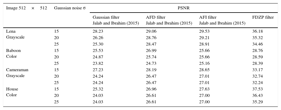
For quantitative comparison purposes, we measured PSNR. It can be seen from Table 1 that the PSNR can be obtained between the original and the denoised image. The original image is corrupted by the additive white Gaussian noise having different standard deviations σ=15, 20, 25. The values obtained for PSNR at different noise standard deviations are shown in Table 1.
Comparison of PSNR obtained by different image denoising filters.
| Image 512×512 | Gaussian noise σ | PSNR | |||
|---|---|---|---|---|---|
| Gaussian filter Jalab and Ibrahim (2015) | AFD filter Jalab and Ibrahim (2015) | AFI filter Jalab and Ibrahim (2015) | FDZP filter | ||
| Lena Grayscale | 15 | 28.23 | 29.06 | 29.53 | 36.18 |
| 20 | 26.26 | 28.76 | 29.21 | 35.32 | |
| 25 | 25.30 | 28.47 | 28.91 | 34.46 | |
| Baboon Color | 15 | 25.53 | 26.99 | 25.66 | 28.76 |
| 20 | 24.87 | 25.74 | 25.66 | 28.59 | |
| 25 | 23.82 | 24.73 | 25.16 | 28.39 | |
| Cameraman Grayscale | 15 | 27.23 | 28.19 | 28.65 | 33.17 |
| 20 | 24.24 | 26.47 | 27.01 | 32.74 | |
| 25 | 24.24 | 26.47 | 27.01 | 32.24 | |
| House Color | 15 | 25.32 | 26.96 | 27.63 | 37.53 |
| 20 | 24.03 | 26.61 | 27.00 | 36.43 | |
| 25 | 24.03 | 26.61 | 27.00 | 35.29 | |
In the experiments, the grayscale images (Lena, Cameraman) are corrupted by the Gaussian noise having different standard deviations σ=15, 20, 25. For the descriptive analysis, to check the performance of the FDZP 2D filter, the variations of PSNR with different σ are shown in Figure 10.
4.3.2Color Images
In the experiments, the color images (Baboon, House) are corrupted by the Gaussian noise having different standard deviations σ=15, 20, 25. To analyze the performance of the FDZP 2D filter, the variations of PSNR with different σ are shown in Figure 10.
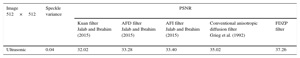
Table 2 gives the comparison of different denoising filters with the proposed FDZP filter for ultrasonic images corrupted by speckle noise in terms of PSNR. The PSNR value for the proposed FDZP filter is much better than other denoising filters shown in Table 2.
Comparison of PSNR obtained by different image denoising methods for an ultrasonic image.
| Image 512×512 | Speckle variance | PSNR | ||||
|---|---|---|---|---|---|---|
| Kuan filter Jalab and Ibrahim (2015) | AFD filter Jalab and Ibrahim (2015) | AFI filter Jalab and Ibrahim (2015) | Conventional anisotropic diffusion filter Grieg et al. (1992) | FDZP filter | ||
| Ultrasonic | 0.04 | 32.02 | 33.28 | 33.40 | 35.02 | 37.26 |
The PSNR value of the proposed FDZP 2D filter is achieved 37.26, which is better as compared to kuan, AFD, AFI and conventional anisotropic diffusion filters. It is clearly observed that the proposed FDZP filter effectively suppresses the noise from the corrupted image.
5ConclusionIn this paper, a FDZP 2D filter is proposed which denoises the corrupted image effectively. From the analysis point of view, our proposed FDZP 2D filter renders a better denoising performance in terms of visual perception and by measuring the PSNR value. The experiments show that the improved result achieved is much better in comparison with standard Gaussian smoothing, AFI and AFD filters, respectively. An additional interesting property of our proposed FDZP 2D filter is characteristic of the denoising algorithm that can be adjusted easily by changing two values of fractional powers of the proposed mask windows. In future work, the proposed FDZP 2D filter technique will be further extended to denoise an image more effectively and also an algorithm will be designed for texture enhancement.
Conflict of interestThe authors have no conflicts of interest to declare.
Peer Review under the responsibility of Universidad Nacional Autónoma de México.