A parallel computing strategy for Monte Carlo simulation using groundwater models

Resumen

En este artículo se presentan los resultados de una estrategia de paralelización para reducir el tiempo de ejecución al aplicar la simulación Monte Carlo con un gran número de realizaciones obtenidas utilizando un modelo de flujo y transporte de agua subterránea. Desarrollamos un script en Python usando mpi4py, a fin de ejecutar GWMC y programas relacionados en paralelo aplicando la biblioteca MPI. Nuestro enfoque consiste en calcular las entradas iniciales para cada realización y correr grupos de estas realizaciones en procesadores separados y después calcular el vector medio y la matriz de covarianza de las mismas. Esta estrategia se aplicó al estudio de un acuífero simplificado en un dominio rectangular de una sola capa. Presentamos los resultados de aceleración y eficiencia para 1000, 2000 y 4000 realizaciones para diferente número de procesadores. Eficiencias de 0,70, 0,76 y 0,75 se obtuvieron para 64, 64 y 96 procesadores, respectivamente. Observamos una mejora ligera del rendimiento a medida que aumenta el número de realizaciones.

Abstract

In this paper we present the results of a parallelization strategy to reduce the execution time for applying Monte Carlo simulation with a large number of realizations obtained using a groundwater flow and transport model. We develop a script in Python using mpi4py, in order to execute GWMC and related programs in parallel, applying the MPI library. Our approach is to calculate the initial inputs for each realization, and run groups of these realizations in separate processors and afterwards to calculate the mean vector and the covariance matrix of them. This strategy was applied to the study of a simplified aquifer in a rectangular domain of a single layer. We report the results of speedup and efficiency for 1000, 2000 and 4000 realizations for different number of processors. Efficiencies of 0.70, 0.76 and 0.75 were obtained for 64, 64 and 96 processors, respectively. We observe a slightly improvement of the performance as the number of realizations is increased.

Introduction

Stochastic hydrogeology is a field that deals with stochastic methods to describe and analyze groundwater processes (Renard, 2007). An important part of it consists of solving stochastic models (stochastic partial differential equations) describing those processes in order to estimate the joint probability density function of the parameters (e.g., transmissivity, storativity) and/or state variables (e.g., groundwater levels, concentrations) of those equations or more commonly some of their moments. Monte Carlo simulation (MCS) is an alternative for solving these stochastic models, it is based on the idea of approximating the solution of stochastic processes using a large number of equally likely realizations. For example, the pioneering work on stochastic hydrogeology by Freeze (1975) applies this method.

The large number of realizations required by MCS can be very demanding in computing resources and the computational time can be excessive. Nowadays there exist many parallel computing platforms that can be used to alleviate this problem. Some previous works have focused in this direction, for example Dong et al. (2012) describe a parallelization strategy for stochastic modeling of groundwater systems using the Java Parallel Processing Framework (JPPF). This tool is very powerful and can be used as a GRID middle-ware (Foster et al., 2001) to distribute tasks across several computing systems. Dong et al. (2012) take advantage of this tool to avoid any modification of MODFLOW and related programs. However, when the JPPF is used in a cluster alone, a simply master-worker parallel model is obtained. They also report that the combination of two levels of parallelism, using a parallel solver to reduce the execution time by an order of two. However, this technique pays off only for very large grids, over 10⁶ points. In our case, we do not require such massive grids.

In this paper, we propose a distributed parallel computing method for stochastic modeling with the software Groundwater Monte Carlo (GWMC), a component of the Groundwater Quality Monitoring (GWQMonitor) package (Herrera, 1998). GWMC is used together with an assimilation method called Ensemble Smoother of Herrera (ESH) in order to estimate groundwater contaminant concentration assimilating concentration data. The best known version of Ensemble Smoother was developed by van Leeuwen and Evensen (1996). Herrera de Olivares developed a version of the assimilation method independently, and originally she called it static Kalman filter (Herrera, 1998).

Ground Water Monte Carlo (GWMC)

GWMC is a program written in FORTRAN by Herrera (1998), and subsequently modified by Olivares-Vázquez (2002).

It implements Monte Carlo simulation using a flow and transport simulator in which hydraulic conductivity is a random field and the contaminant concentration at the contaminant source is a time series at each node. Therefore, multiple realizations of those two parameters are obtained and for each realization the flow and transport equations are solved by the Princeton Transport Code (PTC), a finite element simulator (Babu et al., 1993). Finally, different averages of the concentration solutions are calculated to obtain their space-time mean vector and covariance matrix. In this paper, GWMC is parallelized in order to reduce the program execution time.

Methodology

The methodology implemented in this work is as follows:

Step 1. The input files for PTC are generated.

Step 2. The input files for GWMC are generated.

Step 3. A number of realizations of the natural logarithm of the hydraulic conductivity field are generated using the sequential Gau-ssian simulation (SGSIM) program (Deutsch and Journel, 1997). This program generates standard normal simulated values with a given correlation spatial structure on a rectangular mesh.

Step 4. A transformation to get the hydraulic conductivity field (a lognormal field) is calculated for each realization using the Nrm2log program. This program transforms the standard normal values to a normal variable with a given mean and variance and then applies the exponential function to get the lognormal field.

Step 5. For each node at the source of contaminant concentration, the same number of realizations of time series is generated using the RandTS2 program.

Step 6. If the PTC finite element mesh is not equal to the SGSIM rectangular mesh, the SGSIM mesh is mapped into the nearest node of the PTC mesh.

Step 7. The generated hydraulic conduc-tivity realization value is assigned to the corresponding node of the PTC mesh and the hydraulic conductivity PTC files are substituted with the new values.

Step 8. The contaminant concentrations at the source are substituted by the RandTS2 values in the PTC file for the transport boundary conditions.

Step 9. PTC is executed for each conductivity and source concentration realization (PTC solves numerically the flow and transport equation).

Step 10. Adding over the concentration solutions obtained in step 8, an auxiliary vector with the sum of concentrations for each node and time of interest is calculated and an auxiliary matrix with the sum of products of concentrations for each possible pair of space-time positions of interest is calculated.

Step 11. Combining the information contained in the auxiliary vector and the auxiliary matrix the spatiotemporal mean vector and covariance matrix of the contaminant concentration are calculated.

Step 12. The ESH is applied to estimate contaminant concentration.

Steps 6 to 10 are executed by GWMC and steps 3 to 11 are parallelized in this work.

Python - MPI

Python is an interpreter, interactive and extensible programming language used in a wide variety of applications. In particular, for scientific computing there exist many tools that ease the development of computational codes (Milman and Aivazis, 2011). Python can be combined easily with other programming languages, like C, C++ and Fortran, and al-so can be used to exploit high performance computing architectures by using MPI (Message Passing Interface) [Gropp et al., 1999] or CUDA (Compute Unified Device Architecture) [Kirk and Hwu, 2010]. Currently, almost any operating system supports Python in such a way that this programming language provides portability across many computing platforms.

In this work our main objective is to reduce the execution time of the complete process described in section 4. In order to avoid a complete re-design of our codes, written mainly in FORTRAN, we decided to use Python and MPI for Python (MPI4PY) [Dalcin, 2012]. MPI4PY provides an object-oriented approach for MPI which allows us to distribute tasks using Python scripts. In the appendix we describe briefly the scripts developed in this work.

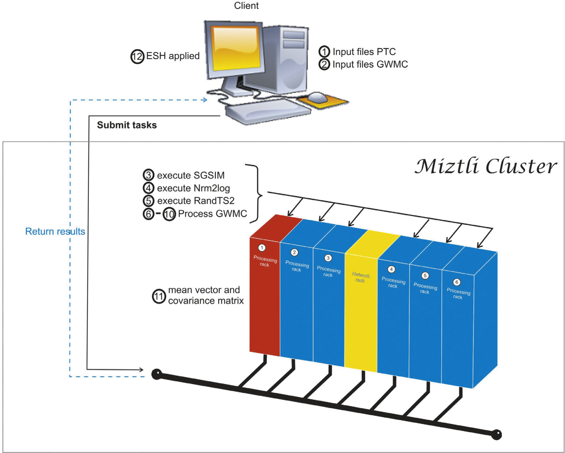
In Figure 1 we sketch the parallelization process. The main idea is to re-use FORTRAN codes with minimal modifications inside a Python script. First, we initialize all the variables and determine the corresponding inputs for the different executable codes. Part of this process is done in a client machine, before the parallel execution. After that, the client submits a batch task to the cluster. Once the parallel execution starts, each processor generates its own input files labeled using the processor number. With the local inputs generated, we execute a group of realizations in each processor. The load balancing is done by the script, distributing the same number of tasks for each processor. Each rea-lization solves the same problem but with different inputs, so the time required by each realization is almost the same. Since the num-ber of realizations can be different for each processor, we need to use a barrier at the end of the parallel execution. However, the waiting time for the last processor is negligible. The calculation of the space-time mean and the covariance matrix is done in processor 1, which requires information from all the processors. Originally, this was done in GWMC. In our case, we removed the corresponding FORTRAN code from the program, and we put it in a separate subroutine that is called at the end of the script. However this change is very simple and straightforward. Finally, the last step (the ESH application) is done as a post processing step in the client machine.

Figure 1.

Parallelization process. Task 3 to 10 are done in parallel, while task 12 is calculated in processor 1.

Application problem

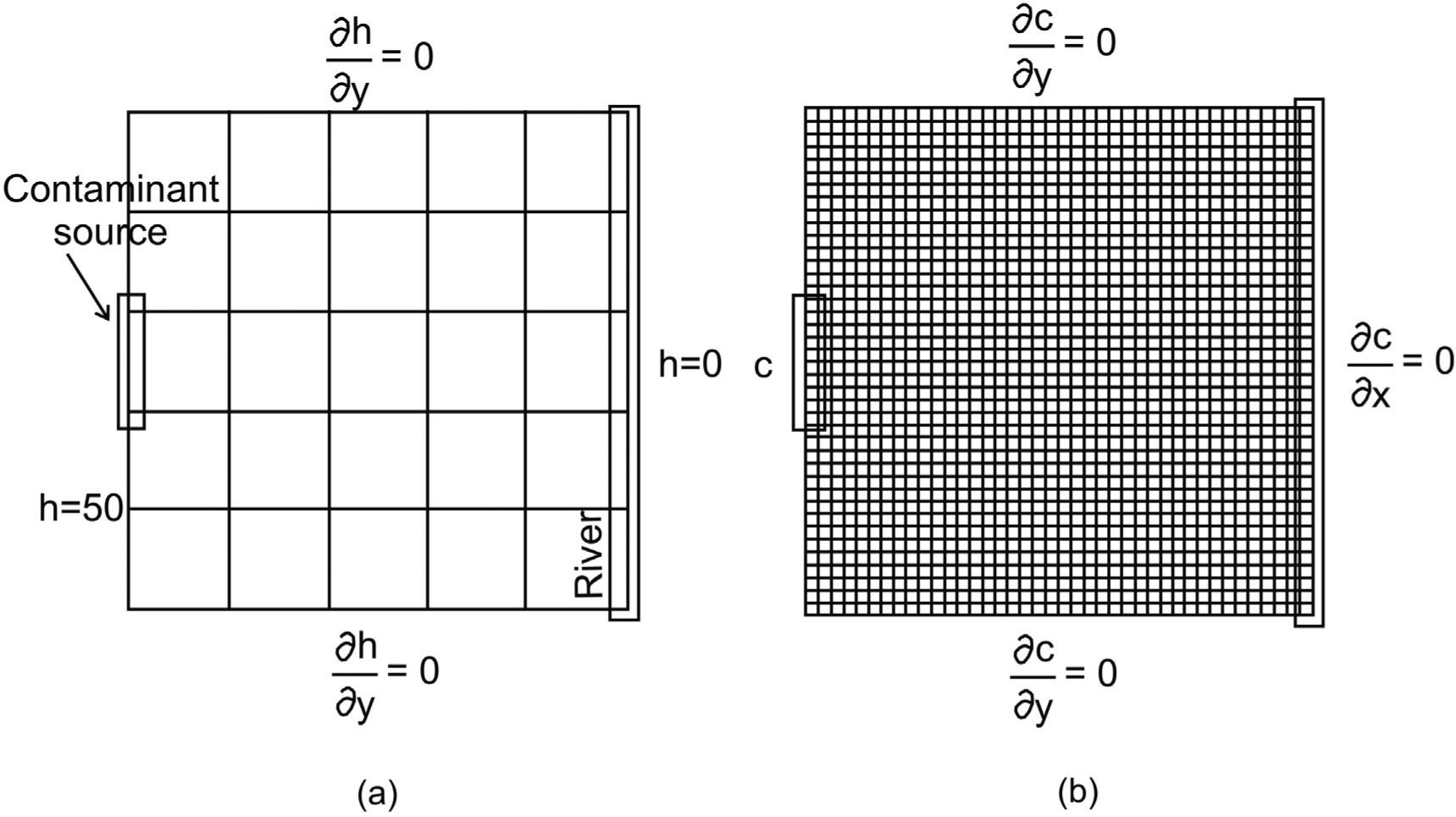
An aquifer of 804.7 by 804.7 m² is considered (figure 2a). A contaminant source is located on the left hand side border and the area is bounded by a river on the right hand side. This problem was slightly modified from the one presented by Herrera and Pinder (2005).

Figure 2.

a) Problem set up with the estimation mesh and boundary conditions for the flow model (h is in meters), b) Stochastic simulation mesh and boundary conditions for the transport model (modified from Olivares-Vázquez, 2002).

The objective is to estimate the contaminant concentrations of a moving plume during a 2-year period. The locations at which concentration estimates will be obtained are associated with the nodes of what we call the estimation mesh shown in Figure 2a. For each one of these locations, concentrations will be estimated every 121.7 days; this amounts to six times during the 2-year period.

Flow and transport model

The PTC is used in two-dimensional mode to solve the flow and transport model. The flow and transport equations coupled through Darcy's law, equations (1), (2) and (3) respectively, are used to describe the contaminant plume evolution:

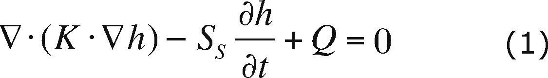
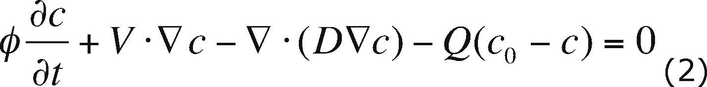
where K is the hydraulic conductivity, h is the hydraulic head, S_S is the specific storage coefficient, Q is a source or sink term, c is the solute concentration, D is the hydrodynamic dispersion, c₀ is the concentration of the pumped fluid and f is the effective porosity. The flow equation (1) describes the water flow through the aquifer; the transport equation (2) describes the changes in contaminant concentration through time for a conservative solute. Darcy's law (3) is used to calculate V, Darcy velocity. Boundary conditions for flow and transport are included in Figures 2a and 2b, respectively. Concentration is given in parts per million (ppm) and hydraulic head in meters (m).

The numerical mesh used to solve the flow and transport equations is called the “stochastic simulation mesh”; it consists of 40x40 equally sized elements (figure 2b). For the transport model forty-eight time-steps are used to simulate a two-year period, 15.2 days each. For the flow model, all nodes of the left hand side boundary have a value of h = 50 m, and all nodes of the right hand boundary have a value of h = 0 m. The contaminant source is active during all of this period, with a constant concentration of c = 50 ppm. Nodes that are not part of the contaminant source satisfy the condition ∂c∂x=0 The aquifer is assigned a thickness of 55 m, a porosity of 0.25, a dispersivity of 33 m in the x direction and 3.3 m in the y direction.

Stochastic model

As was mentioned before, the hydraulic conductivity is represented as a spatially correlated random field; thus, the resulting velocity and dispersion fields, also become spatially correlated random fields.

For this example we will assume that the hydraulic conductivity field has a lognormal distribution, it is homogeneous, stationary and isotropic. The mean value of F(x) = 1nK(x) is 3.055 and the semivariogram that represents its spatial correlation structure is an exponential model, i.e.:

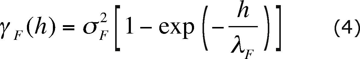
where σ2F is the variance of F with value 0.257813, and λ_F is its correlation scale equal to 80.467 m.

At each node the contaminant concentration is represented as a time series (Herrera and Pinder, 2005), through

where e(t) is a zero-mean random perturbation, normally distributed and with a 0.1948 variance. For each source node, in every simulation time step, a different random perturbation is used. The time correlation of the random perturbations is modeled with the semivariogram

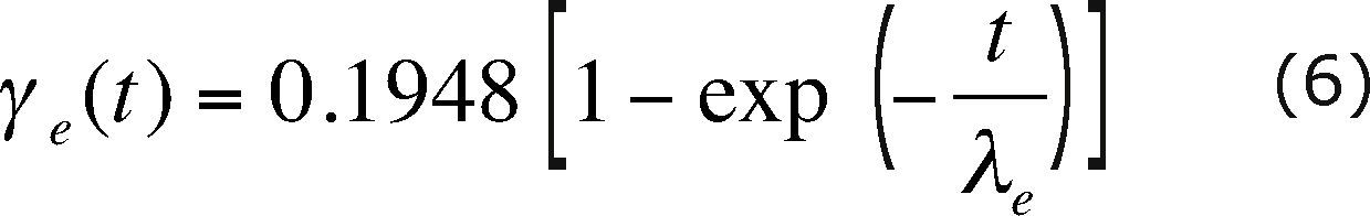
with λ_e equal to 11 days.

For this example we used 1000, 2000 and 4000 realizations.

Estimation with the Ensemble Smother of Herrera (ESH)

As was mentioned before, Herrera (1998) developed the assimilation method independently of van Leeuwen and Evensen (1996), it was called static Kalman filter and later, static ensemble Kalman filter (EnKF) by Nowak et al. (2010).

Using the ESH we estimate the conservative contaminant concentration using existing da-ta for a two-year period. The concentration estimates are obtained at the nodes of what we call the ESH-mesh, which is a submesh of the stochastic simulation mesh, which consists of 5x5 equally sized elements (this mesh is shown in figure 2a). For each of these positions, the concentrations are estimated six times over a period of two years, equivalent to 121.7 days. To apply the ESH it is necessary to calculate the space-time covariance matrix of the contaminant concentration.

Performance

We execute our codes on a HP Cluster Platform 3000SL “Miztli”, consisting of 5,312 processing cores Intel E5-2670, 16 cards NVIDIA m2090, with 15,000 GB of RAM, and capable of processing up to 118 TFlop/s. The system has 750 TB of massive storage.

Parallel metrics

Some of the most commonly used metrics to determine the performance of a parallel algorithm are the speedup and efficiency.

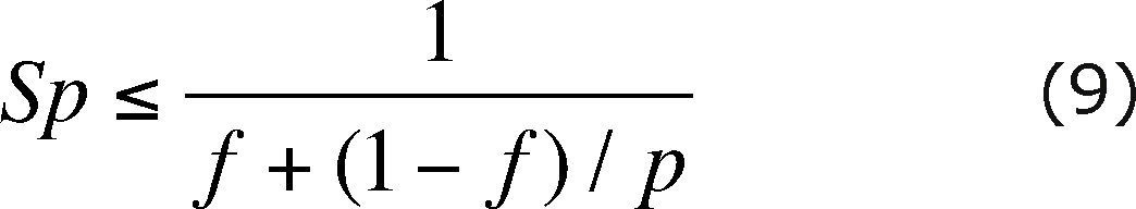
The speedup (S_p) is defined as

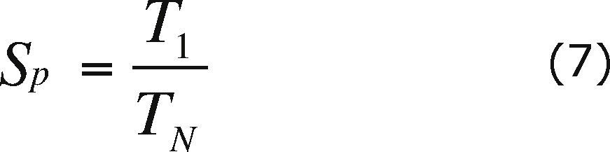
where T₁ is the running time of the algorithm on one processor and T_N is the running time of the algorithm on N processors.

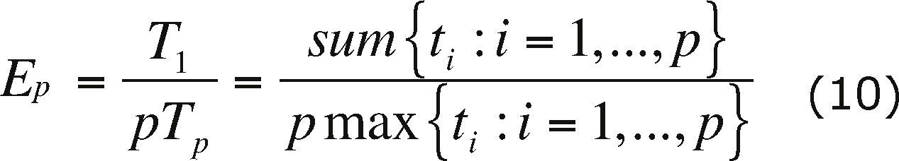
The efficiency (E_p) is defined as

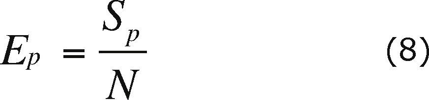
where N is the number of processors in which the algorithm execution is carried out.

In this paper, these metrics are used to verify how efficient is the parallelization of GWMC.

The serial execution of GWMC for one thousand realizations took on average 24.5 minutes using PTC to solve the flow and transport equations.

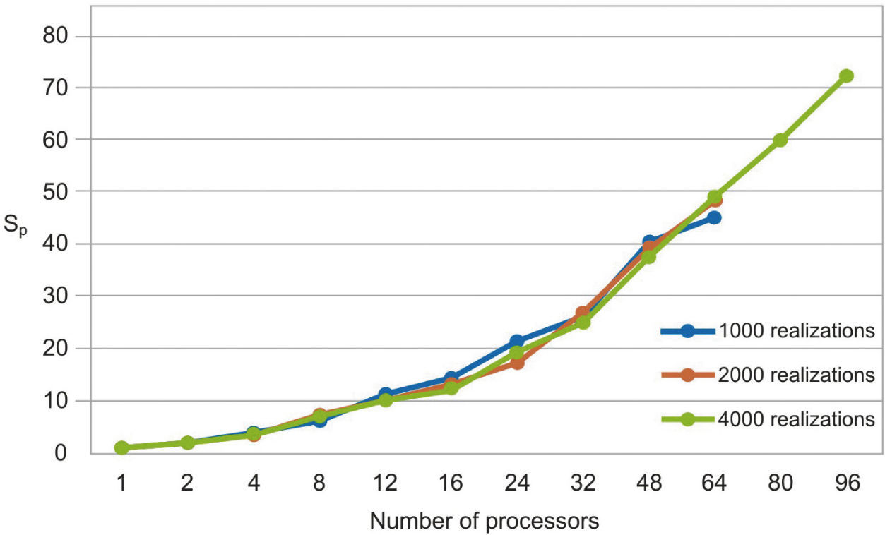
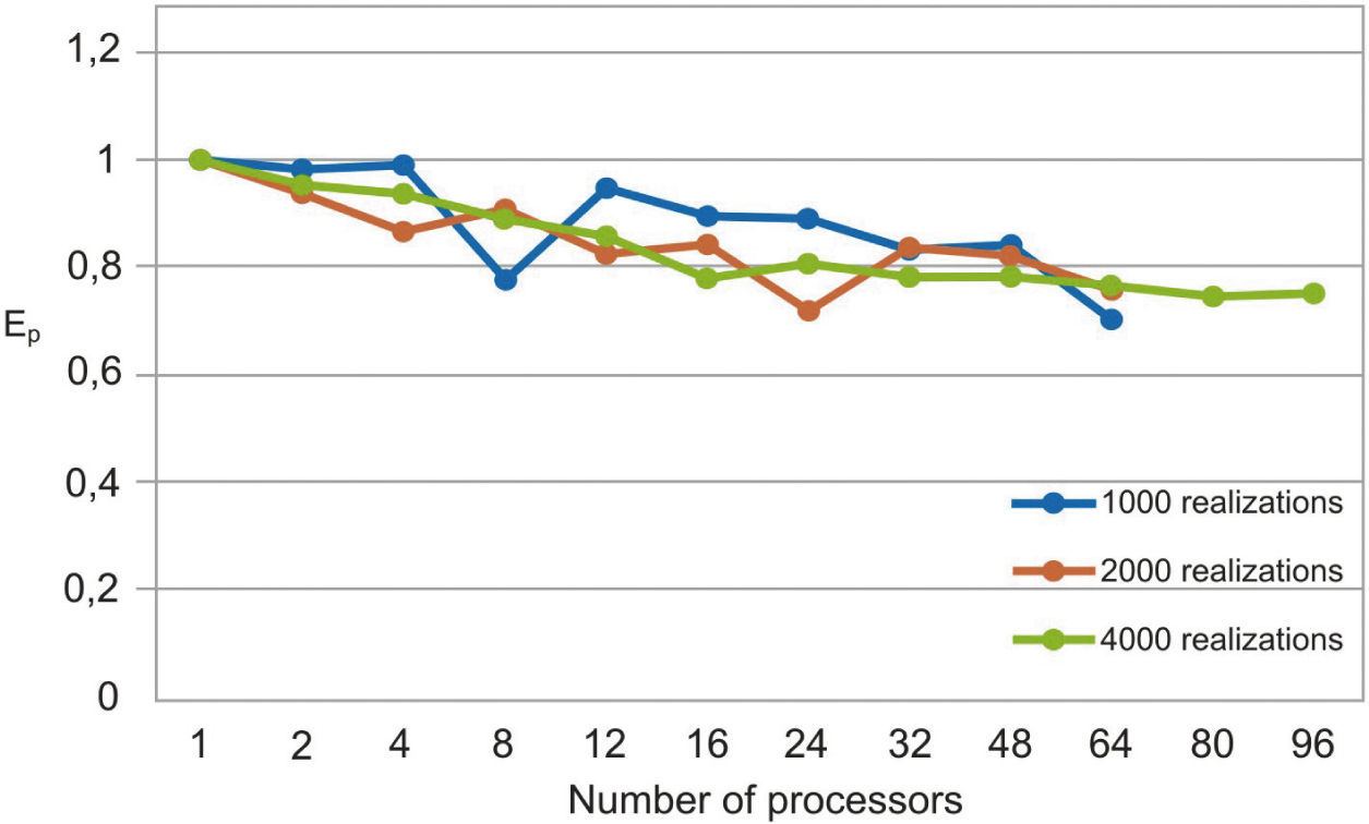
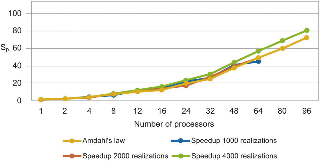
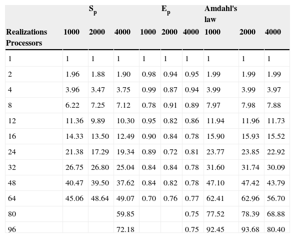
The parallel Python script was executed for 1000, 2000 and 4000 realizations with different numbers of processors (see Table 1). We observe that the speedup grows when the number of processors increases (figure 3). In Figure 4 we see that the efficiency is more stable for the 4000 realizations case since it has fewer oscillations. For the 1000 realizations case, a speedup of 45.06 was obtained with 64 processors and a correspondingly efficiency of 0.70; for the 2000 realizations case, a speedup of 48.64 was obtained with 64 processors and a correspondingly efficiency of 0.76; for the 4000 realizations case, a speedup of 72.18 was obtained with 96 processors and a correspondingly efficiency of 0.75. The number of realizations has not much effect in the speedup and efficiency, since their values for the three cases for the same number of processors are similar.

Table 1.

Speedup (Sp), efficiency (Ep) and Amdahl's law data with different number of processors for 1000, 2000 and 4000 realizations.

		Sp			Ep		Amdahl's law
Realizations Processors	1000	2000	4000	1000	2000	4000	1000	2000	4000
1	1	1	1	1	1	1	1	1	1
2	1.96	1.88	1.90	0.98	0.94	0.95	1.99	1.99	1.99
4	3.96	3.47	3.75	0.99	0.87	0.94	3.99	3.99	3.97
8	6.22	7.25	7.12	0.78	0.91	0.89	7.97	7.98	7.88
12	11.36	9.89	10.30	0.95	0.82	0.86	11.94	11.96	11.73
16	14.33	13.50	12.49	0.90	0.84	0.78	15.90	15.93	15.52
24	21.38	17.29	19.34	0.89	0.72	0.81	23.77	23.85	22.92
32	26.75	26.80	25.04	0.84	0.84	0.78	31.60	31.74	30.09
48	40.47	39.50	37.62	0.84	0.82	0.78	47.10	47.42	43.79
64	45.06	48.64	49.07	0.70	0.76	0.77	62.41	62.96	56.70
80			59.85			0.75	77.52	78.39	68.88
96			72.18			0.75	92.45	93.68	80.40

Figure 3.

Speedup versus number of processors for 1000, 2000 and 4000 realizations.

Figure 4.

Efficiency versus num-ber of processors for 1000, 2000 and 4000 realizations.

Discussion

The elapsed time, the speedup and efficiency are limited by several factors: serial fraction of the code, load balancing, data dependencies and communications. In our case we have a minimal part of serial section: at the very beginning of the code, when the problem is set up in each processor; and at the end of the code when we join the results of all processors to calculate the mean vector and the covariance matrix. We have a very good load balancing due to the fact that each processor works on the same number of realizations. There are not data dependencies during calculations, except for the mean vector and covariance matrix calculations. Finally, the communications required to complete the calculations are also at the beginning and at the end of the code.

Almost all the factors that limit the efficiency of our code, can be taken in to account in the serial fraction, because are present at the beginning and the end of the code, i.e. during the serial part of the execution. Therefore, using Amdahl's law (Ridgway et al., 2005) we can predict the theoretical maximum speedup of the code beforehand. Amdahl's law formula is

where f represents the sequential fraction of the code and p is the number of processors.

The serial fraction is measured in time units, therefore, when we increase the number of realizations, the processors will have more work to do in parallel reducing the serial fraction as a consequence. This effect can be seen in the results presented in Table 1 and in Figures 3 and 4, where the speedup and the efficiency are more stable when the number of realizations is increased.

In figure 5, we compare our speedup results against Amdahl's law drawn for 4000 realizations. We observe that our results for the three cases are in very good agreement with the predictions of this law. The mean squared errors of our results, compared with the Amdahl's law, are 1.95, 1.86 and 1.43 for 1000, 2000 and 4000 realizations, respectively, which proofs also the effectiveness of our approach. Besides, the efficiencies obtained are also greater than 0.70, in such a way that our parallel codes are scalable (see Ridgway et al., 2005).

Figure 5.

The comparative bet-ween the Amdahl's law and the speedup to 1000, 2000 and 4000 realizations.

Amdahl's law assumes a perfect load balancing. The definition of load balancing is in terms of the time t_i that each processor takes in its calculations during the parallel part. A good balancing is when all the t_i's have the same value approximately. In terms of these t_i's the parallel time of the code will be T_p = max{t_i : i = 1, ..., p}. It is reasonable to assume that the time of the whole process in one processor is T₁ = sum{t_i : i = 1, ..., p}. Then using the efficiency we have:

Therefore, we can write

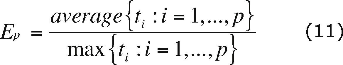
Hence, if the load balancing is bad, then the max{t_i : i = 1, ..., p} will be high, reducing the efficiency and speedup. In our case, we distribute the realizations on the processors evenly, producing averages and a maximum, of t_i : i = 1, ..., p, with very similar values.

Another important aspect in parallel applications is the communication between processors. In the cluster we used, the connections between processing nodes is based on Infiniband QDR 40 Gigabits per second technology. This network reduce drastically the communications time of our codes, besides we do not use exchange of information once the parallel process is initiated, only at the setup of the problem and at the end of the calculations. We also tested the same codes on a cluster with Ethernet interconnection but the results were not as good as with those obtained with the Infiniband technology.

Conclusions

In this paper, a parallelization strategy for Monte Carlo-type stochastic modeling, with PTC-related programs, has been described. The software GWMC implements this process for one processor. Our strategy allows us to re-use all these codes, with minimal modifications.

The results obtained in parallel show that the performance is more stable as the workload for each processor is increased. In particular we obtained a very good efficiency for 4000 realizations and 96 processors. In this case we have an efficiency of 0.75 which makes our codes scalable and useful for large scale applications. During the development of this work, we have not installed any complicated software, we just use the common libraries installed in the Miztli cluster. In addition, we made a very simple modification of our original FORTRAN code to calculate the global covariance matrix.

We believe that our strategy is simple but effective for a large number of simulations and can be applied to study more complicated problems, where the execution times can be very large.

We show in Figure 5 that the speedup of 1000, 2000 and 4000 realizations has a good load balancing, because the Amdahl's law assumes a perfect load balancing, and the speedup meets the conditions described in the discussion section, for this reason, we assume that our speedup had a good load balancing.

Appendix

In what follows we describe parts of the script written to parallelize the process described in section 4.

1) A first step is to create directories to facilitate the parallelization and storing of the information. We use the rank of the processor to define the name of each directory:

if os.path.isdir(‘%s’ % t + ‘%d’ % rank):

shutil.rmtree(‘%s’ % t + ‘%d’ % rank)

os.mkdir(‘%s’ % t + ‘%d’ % rank)

os.chdir(‘%s’ % t + ‘%d’ % rank)

2) Four input files need to be modified, these are: gwqmonitor.par, sgsim.par, nrm2log.par and randTS2.par. Each file contains inputs for codes rndcsim, sgsim, nrlm2log and randTS2 respectively. Modification of file sgsim.par is shown below:

ofile = open(“sgsim.par”, ‘w’)

i=0

for line in lines:

i+=1

if i==21:

ofile.write(‘%d \n’ % local_realizaciones)

elif i==25:

j+=2

ofile.write(‘%d \n’ % j)

else:

ofile.write(‘%s’ % line)

ofile.close()

3) All input files are copied in each cluster node in order to run the programs sgsim, nrm2log, randTS2 and GWQMonitor. Once the copy of the input files is done, we execute each one of these programs. Note that the FORTRAN executable codes are run using a system call from the python script:

os.system(‘./sgsim < sgsim.par > sgsim.OUTPY’)

os.system(‘./nrm2log > nrm2log.OUTPY’)

os.system(‘./randts2 > randts2.OUTPY’)

os.system(‘./gwqmonitor > gwqmonitor.OUTPY’)

4) For the calculation of the covariance matrix, we use a barrier to ensure that the information from the different processors has been arrived to the memory of processor that construct the covariance matrix. Calculation of the covariance matrix is carried out after this information is gathered.

MPI.COMM_WORLD.Barrier()

if (rank==0):

def checkfile(archivo):

import os.path

if os.path.isfile(archivo):

os.system(‘rm %s’%archivo)

os.chdir(‘/home/estherl/NV3-MPI/’)

checkfile(‘covarianza.out’)

checkfile(‘media.out’)

print(“tiempo sgsim = %e’ % (t2-t1))

print(“tiempo nrmlog = %e’ % (t3-t2))

print(“tiempo randts2 = %e’ % (t4-t3))

print(“tiempo gwqmonitor = %e’ % (t5-t4))

os.system(‘./matriz %d’ %size)

os.system(‘mv meanvect*.out basura/’)

os.system(‘mv meanplume*.out basura/’)

os.system(‘mv covmatrx*.out basura/’)

Observe that the steps 1) to 4) are all executed by all processors in parallel; it is only using the rank of each processor that is possible to assign different tasks to each processor. Actually, this latter is done in the step 4).

Acknowledgements

The authors gratefully acknowledge Leobardo Itehua for helping us running the numerical tests in Miztly and E. Leyva the scholarship from CONACyT to pursue her Ph.D. studies.