


This study aims to develop a Bayesian methodology to identify, quantify and measure operational risk in several business lines of commercial banking. To do this, a Bayesian network (BN) model is designed with prior and subsequent distributions to estimate the frequency and severity. Regarding the subsequent distributions, an inference procedure for the maximum expected loss, for a period of 20 days, is carried out by using the Monte Carlo simulation method. The business lines analyzed are marketing and sales, retail banking and private banking, which all together accounted for 88.5% of the losses in 2011. Data was obtained for the period 2007–2011 from the Riskdata Operational Exchange Association (ORX), and external data was provided from qualified experts to complete the missing records or to improve its poor quality.
Esta investigación tiene como propósito desarrollar una metodología bayesiana para identificar, cuantificar y medir el riesgo operacional en distintas líneas de negocio de la banca comercial. Para ello se diseña un modelo de red bayesiana con distribuciones a priori y a posteriori para estimar la frecuencia y la severidad. Con las distribuciones a posteriori se realiza inferencia sobre la máxima pérdida esperada, para un período de 20días, utilizando el método de simulación Monte Carlo. Las líneas de negocio analizadas son comercialización y ventas, banca minorista y banca privada, que en conjunto representaron el 88,5% de las pérdidas en 2011. Los datos fueron obtenidos de la Asociación Riskdata Operacional Exchange (ORX) para el período 2007-2011, y la información externa fue proporcionada por expertos calificados para completar los registros faltantes o mejorar los datos de mala calidad.
Esta pesquisa tem como objetivo desenvolver uma metodologia Bayesiana para identificar, quantificar e medir o risco operacional em diversas linhas de negócio da banca comercial. Isso requer (e é projetado) um modelo de Rede Bayesiana (RB), com distribuições anteriores e posteriores para estimar a frequência e a severidade. Com as distribuições posteriores é realizada una inferência sobre a perda máxima esperada por um período de 20 dias, usando o método de simulação de Monte Carlo. As linhas de negócio analisadas são marketing e vendas, banca de retalho e banca privada, que juntos representaram 88,5% das perdas em 2011. Os dados foram obtidos a partir da Associação Riskdata Operacional Exchange (ORX) para o período 2007-2011, e a informação externa foi fornecida por peritos qualificados para completar os registros ausentes ou melhorar os dados de má qualidade.
While in 2004 regulators focused on market, credit and liquidity risk, in 2011 attention was mainly placed on the high-profile loss events affecting several major financial institutions, which renewed operational risk management and corporate governance. For global markets, the significance of loss events (measured, in some cases, in billions of dollars) showed that the lack of an appropriate operational risk management may affect even major financial institutions.
The current challenge is how to manage proactively operational risk in a business environment characterized by sustained volatility. Needless to say financial organizations need advanced tools, models, techniques and methodologies that combine internal data with external data across industry. For example, organizations in the banking and insurance sectors can provide critical insights from self-assessment and scenario modeling from the combination of internal data with external data on loss events that triggers across the industry. External loss event data not only provides insights from the experiences of industry peers, but also allows a more effective identification of potential risk exposure. For increasing effectiveness in analyzing potential risk exposure, predictive indexes and indicators combining internal and external data may be developed for a more effective operational risk management. These predictions will lead to a more accurate evaluation of potential future losses.
The Bayesian approach may be an appropriate alternative for operational risk analysis when initial and/or complementary information from qualified consultants is available. By construction, Bayesian models incorporate initial or complementary information about parameter values of a sampling distribution through a prior probability distribution, which includes subjective information provided by expert opinions, analyst judgments or specialist beliefs. Subsequently, a posterior distribution is estimated to carry out inference on the parameter values. This paper develops a Bayesian Network (BN) model to examine the relationships among operational risk (OR) events in the three lines of business with greater losses in the international banking sector. The proposed BN model is calibrated with observed data from events occurred in these lines of business and/or with information obtained from experts or from external sources.1 In this case, experts mainly complete missing records or improve data of poor quality. The analysis period for this research is from 2007 to 2011 on the basis of a twenty-day frequency. This period starts one year before the financial crisis generated by subprime mortgages.
OR usually involves a small part of total annual losses from commercial banks; however, at the time an extreme event of operational risk occurs, it can cause significant losses. For this reason, major changes in the worldwide banking industry are aimed at having better policies and recommendations concerning operational risk. It is noteworthy that exist in the literature various statistical techniques to identify and quantify OR, which have the underlying assumption of independence between risk events; see, for example: Degen, Embrechts, and Lambrigger (2007), Moscadelli (2004), Embrechts, Furrer, and Kaufmann (2003). However, as shown in Aquaro et al. (2009), Supatgiat, Kenyon, and Heusler (2006), Carrillo-Menéndez and Suárez-González (2015), Carrillo-Menéndez, Marhuenda-Menéndez, and Suárez-González (2007), Cruz (2002), Cruz, Peters, and Shevchenko (2002), Neil, Marquez, and Fenton (2004) and Alexander (2002) there is a causal relationship between OR factors.
Despite the research from Reimer and Neu (2003, 2002), Kartik and Reimer (2007), Aquaro et al. (2009), Neil et al. (2004) and Alexander (2002), that apply the BN scheme in OR management, there is no a complete guide on how to classify, identify, quantify OR events, and how to calculate economic capital consistently.2 This work aims to close these gaps. First, establishing OR event information structures so that it is possible to quantify the OR events and then changing the assumption of independence of events in order to model more realistically the causality relationship of OR events.
The possibility of using conditional distribution (discrete or continuous), calibrating the model with both objective and subjective information sources, and establishing causal relationships among risk factors, is precisely what distinguishes our research compared with classical statistical models. Under this framework, this paper is aimed at calculating, with several confidence levels, the maximum expected loss over a period of 20 days for the group of international banks associated to the ORX regarding the studied lines of business of commercial banks, which has to be considered to properly manage operational risk in ORX.
This paper is organized as follows. Section 2 presents the typology to be used for OR management in accordance with the Data Operational Riskdata eXchange Association (ORX). Section 3, briefly, reviews the main methods, models and tools for measuring OR. Section 4 discusses the theoretical framework needed for the development of this research, emphasizing on the advantages and benefits of using BNs. Section 5 provides two BN, one for frequency and other for severity. In order to quantify the OR at each node of the network, we fit prior distributions by using the @Risk software. Once the prior probabilities of both networks are estimated, we proceed to calculate posterior probabilities and, subsequently, we use the junction tree algorithm to eradicate cycles when the directionality is eliminated (See Appendix). Section 6 combines prior and posterior distributions to compute the loss distribution by using Monte Carlo simulation. Here, the maximum expected loss arising from operational risk events for a period of 20 days is calculated. Finally, we present conclusions and acknowledge limitations.
2Operational risk events in the international banking sectorThis section describes, in some detail, the operational risk events related to the international banking sector according with the Data Operational Riskdata eXchange Association (ORX).
- •
External frauds
We describe now the operational risk events related to external fraud according to ORX:
- a)
Fraud and theft: these are losses due to a fraudulent act, misappropriate property, or law circumvent, by a third party without the assistance of the bank staff.
- b)
Security systems: this applies to all events related to unauthorized access to electronic data files.
- a)
- •
Internal frauds
The operational risk events related to internal fraud are described below:
- a)
Fraud and theft: losses due to fraudulent acts, improper appropriations of goods, or evasion of regulation or company policy, that involves the participation of internal staff.
- b)
Unauthorized activities: losses caused from unreported intentional and unauthorized operations, or intentionally unregistered positions.
- c)
Security systems: this previous category applies to all events involving unauthorized access to electronic data files for personal profit with the assistance of employee's access.
- a)
- •
Malicious damage
Losses caused by acts of badness or hatred, in others words malicious damage.
- a)
Deliberate damage: this is concerned with acts of vandalism, excluding events in security systems.
- b)
Terrorism: ill-intentioned damage caused by terrorist acts excluding events related to security systems.
- c)
Security systems (external): these events include security events with deliberate damage in external systems made by a third party without the assistance of internal staff (e.g., the spread of software viruses).
- d)
Security systems (internal): this includes deliberate events in the security of internal systems with the participation of internal staff (e.g., the spread of software viruses).
- a)
- •
Labor practices and workplace safety
Labor practices and safety at workplace are losses derived from actions not in agreement with labor, health or safety regulation. Payment claims for bodily injury or loss of discriminatory events. Mandatory insurance programs for workers and regulation on safety in the workplace are included in this category.
- •
Customers, products and business practice
Business practices, these events consider losses arising from an unintentional or negligent breach of a professional obligation to specific clients or the design of a product, including fiduciary and suitability requirements.
- •
Disasters and accidents
Disasters and accidents reflects losses resulting from damage to physical assets from natural disasters, or other events like traffic accidents.
- •
Technology and infrastructure failure
Losses caused by failures in systems or management.
- a)
Failures in technology and infrastructure, such as hardware, software and telecommunications malfunctioning.
- b)
Failures in management processes.
- a)
Operational risk management usually involves a small part of total annual losses from international banks; however, when an unexpected extreme event, that occasionally occurs, may cause significant losses. For this reason, major changes in the worldwide banking industry are aimed at obtaining better policies and/or recommendations concerning with operational risk management. Financial globalization and local regulation leads us also to rethink and reorganize operational risk associated to international banking, including those too big to fail. In this sense, a suitable operational management in the international banking sector may avoid possible bankruptcy and contagion and, therefore, systemic risk. The available approaches to deal with this issue vary from simple to highly complex methods with very sophisticated statistical models. Now, we briefly describe some of the existing methods in the literature for measuring OR; see, for example, Heinrich (2006) and Basel II (2001a, 2001b). It will be also emphasized in this subsection on the advantages and benefits of using BN.
- 1)
The “top-down” single indicator methods. These methods were chosen by the Basel Committee as a first approach to operational risk measurement. A single indicator of the institution as total income, volatility of income, or total expenditure, can be considered as the functional variable to manage the risk.
- 2)
The “bottom-up” models including expert judgment. The basis for an expert analysis is a set of scenarios. In this case, experts mainly complete missing records or improve data of poor quality of the identified risks and their probabilities of occurrence in alternative scenarios.
- 3)
Internal measurement. The Basel Committee proposes the internal measurement approach as a more advanced method for calculating the regulatory capital.
- 4)
The classical statistical approach. This framework is similar to what is used in the quantification methods for market risk, and more recently the credit risk. However, contrary to what happens with market risk, it is difficult to find a widely accepted statistical method.
- 5)
Causal models. As an alternative to the classical statistical framework, causal models assume dependence in the occurrence of OR events. Under this approach, each event represents a random variable (discrete or continuous) with a conditional distribution function. In case that the events have no historical records or data has poor quality, it is required the opinion or judgment of experts to determine the conditional probabilities of occurrence. The tool for modeling this causality is just the BN, which is based on Bayes’ theorem and the network topology.
In this section the theory supporting the development of the proposed BN is presented. It begins with a discussion of the conditional value at risk (CVaR) as a coherent risk measure in the sense of Artzner, Delbaen, Eber, and Heath (1999). The CVaR will be used to compute the expected loss. Afterward, the main concepts of the BN approach are introduced.
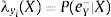
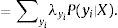
Acording to Panjer (2006), the CVaR or Expected Shortfall (ES) is an alternative measure to Value at Risk (VaR) that quantifies the losses that can be found in the distributions tails. Specifically, let X be the random variable representing the losses, the CVaR of X with a (1−p)×100% confidence level, denoted by CVaR(X), represents the expected loss given that the total losses exceed the 100×p quantile of the distribution of X. Thus, CVaRp (X) can be written as:
where F(x) is the cumulative distribution function of X. Hence, the CVaR(X) can be seen as the average of all the values of VaR with a p×100% confidence level. Finally, notice that CVaR(X) can be rewritten as:where e(xp) is the average excess of loss function.3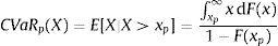

- •
The Bayesian framework
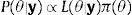
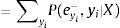
In statistical analysis there are two main paradigms, the frequentist and the Bayesian. The main difference between them is the definition of probability. The frequentist states that the probability of an event is the limit of its relative frequency in the long run. While the Bayesian argue that probability is subjective. The subjective probability (degree of belief) is based on knowledge and experience and is represented through a prior distribution. The subjective beliefs are updated by adding new information to the sampling distribution through Bayes’ theorem obtaining a posterior distribution, which is used to make inferences on the parameters of the sampling model. Thus, a Bayesian decision maker learns and revises its beliefs based on new available information.4 Formally, Bayes’ theorem states that
where θ is a vector of unknown parameters to be estimated, y is a vector of observations recorded, π(θ) is the prior distribution, L(θ|y) is the likelihood function for θ, and P(θ|y) is the posterior distribution of θ. Two main questions arise, how to translate prior information in an analytical form, π(θ), and how to assess the sensitive of the posterior with respect to the prior selection.5A BN is a graph representing the domain of decision variables, its quantitative and qualitative relations and their probabilities. A BN may also include utility functions that represent the preferences of the decision maker. An important feature of a BN is its graphical form, which allows a visual representation of complicated probabilistic reasoning. Another relevant aspect is the qualitative and quantitative parts of a BN, allowing incorporate subjective elements such as expert opinion. Perhaps the most important feature of a BN is that it is a direct representation of the real world and not a way of thinking. Each node is associated with a set of tables of probabilities in a BN. The nodes stand for the relevant variables, which can be discrete or continuous.6 A causal network according to Pearl (2000) is a BN with the additional property that the “parent” nodes are the directed causes.7
A BN is used primarily for inference by calculating conditional probabilities given the information available at each time for each node (beliefs). There are two classes of algorithms for the inference process: the first generates an exact solution and the second produces an approximate solution with high probability to be in close proximity to the exact solution. Among the exact inference algorithms, we have for example: polytree, clique tree, tree junction, algorithms of variable elimination and Pear's method.
The use of approximate solutions is based on the exponential growth of the processing time required to obtain exact solutions. According to Guo and Hsu (2002) such algorithms can be grouped in: stochastic simulation methods, model simplification methods, search based methods, and loopy propagation methods. The best known is the stochastic simulation, which is, in turn, divided in sampling algorithms and Markov Chain Monte Carlo (MCMC) methods.
In what follows, we will be concerned with building the BN for the international banking sector. The first step is to define the problem domain where the purpose of the NB is specified. Subsequently, the important variables and nodes are defined. Then, the interrelationships between nodes and variables are graphically represented. The resulting model must be validated by experts in the field. In case of disagreement between them, we return to one of the above steps until reaching consensus. The last three steps are: incorporate expert opinion (referred to as the quantification of the network), create plausible scenarios with the network (network applications), and finally network maintenance.
The main problems that a risk manager faces when using a BN are: how to implement a Bayesian network, how to model the structure, how to quantify the network, how to use subjective data (from experts) and/or objective (statistical data), what tools should be used for best results, and how to validate the model. The answers to these questions will be addressed in the development of our proposal. Moreover, one of the objectives of this paper is to develop a guide for implementing a NB to manage operational risk in international banking associated with ORX. We also seek to generate a consistent measurement of the minimal capital requirements for managing OR.
We will be concerned with the analysis of operational risk events occurring in the following lines of business: marketing and sales, retail banking and private banking of international banks joined to the Operational Riskdata eXchange Association. Once the risk factors linked with each business line are identified, the nodes that will be part of the Bayesian network have to be defined. They are random variables that can be discrete or continuous and have associated probability distributions. One of the purposes of this research is to compute the monthly maximum expected loss associated to transnational banks belonging to ORX. The frequency of the available data is every twenty days, ranging from 2007 through 2011.
- •
Building and quantifying the model
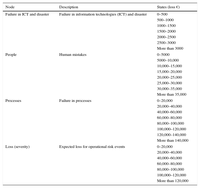
The nodes are connected with directed arcs (arrows) to form a structure that shows the dependence or causal relationship between them. The BN is divided into two networks, one for modeling the frequency and the other for the severity. Once the results are obtained separately, they are aggregated through Monte Carlo simulation to estimate the loss distribution. Usually, the severity network requires a significant amount of probability distributions. In what follows, the characteristics and states of each node of the networks for severity and frequency are described in Tables 1 and 2, respectively.
Table 1.Network nodes for severity.
Node Description States (loss €) Failure in ICT and disaster Failure in information technologies (ICT) and disaster 0–500 500–1000 1000–1500 1500–2000 2000–2500 2500–3000 More than 3000 People Human mistakes 0–5000 5000–10,000 10,000–15,000 15,000–20,000 20,000–25,000 25,000–30,000 30,000–35,000 More than 35,000 Processes Failure in processes 0–20,000 20,000–40,000 40,000–60,000 60,000–80,000 80,000–100,000 100,000–120,000 120,000–140,000 More than 140,000 Loss (severity) Expected loss for operational risk events 0–20,000 20,000–40,000 40,000–60,000 60,000–80,000 80,000–100,000 100,000–120,000 More than 120,000 Source: Own elaboration.
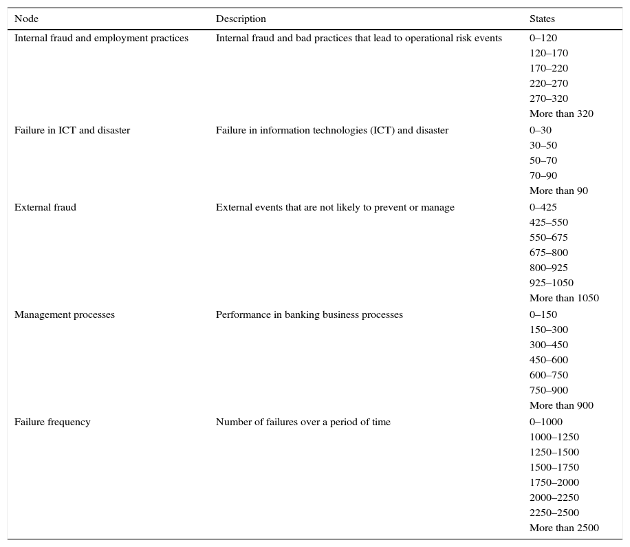
Table 2.Network nodes for frequency.
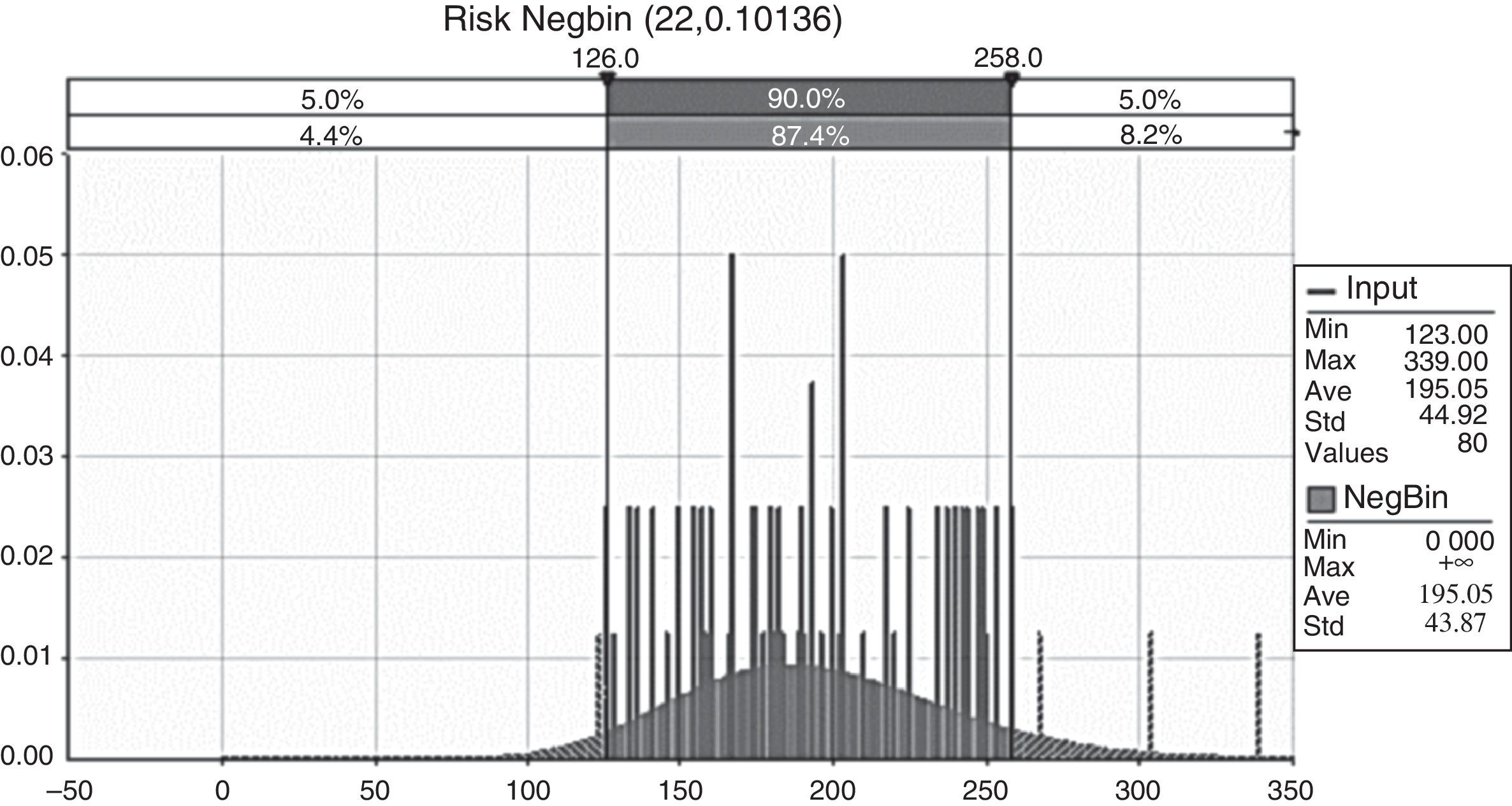
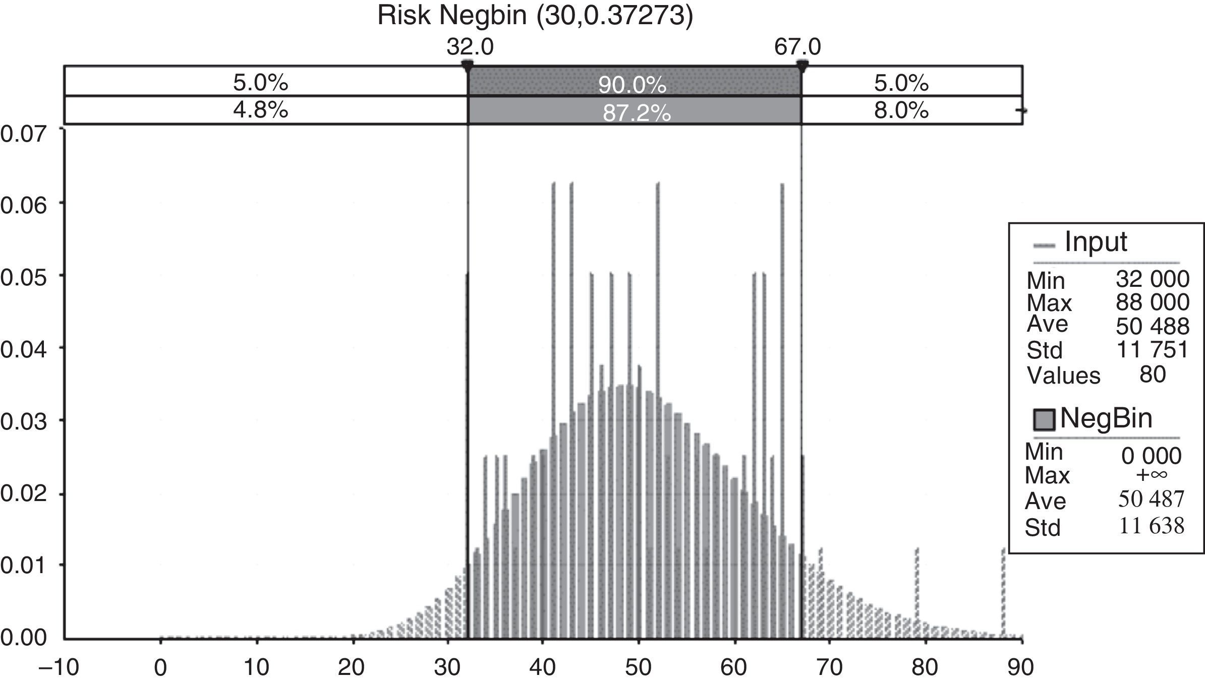
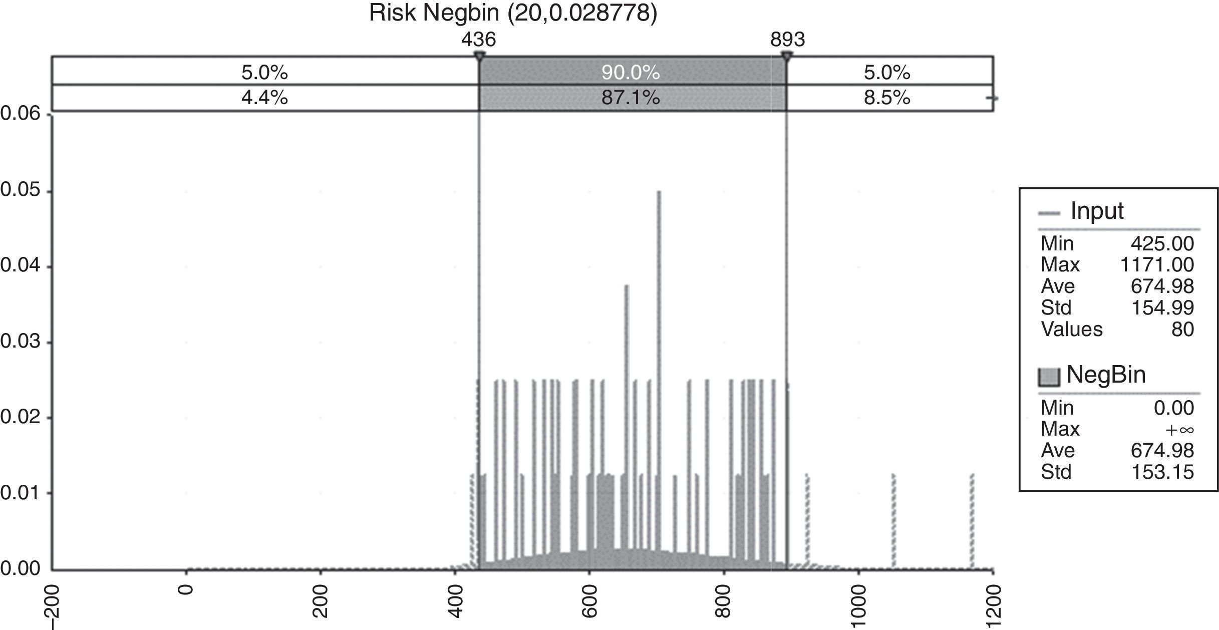
Node Description States Internal fraud and employment practices Internal fraud and bad practices that lead to operational risk events 0–120 120–170 170–220 220–270 270–320 More than 320 Failure in ICT and disaster Failure in information technologies (ICT) and disaster 0–30 30–50 50–70 70–90 More than 90 External fraud External events that are not likely to prevent or manage 0–425 425–550 550–675 675–800 800–925 925–1050 More than 1050 Management processes Performance in banking business processes 0–150 150–300 300–450 450–600 600–750 750–900 More than 900 Failure frequency Number of failures over a period of time 0–1000 1000–1250 1250–1500 1500–1750 1750–2000 2000–2250 2250–2500 More than 2500 Source: Own elaboration.
In the Bayesian approach, the parameters of a sample model are treated as random variables. The prior knowledge about the possible values of the parameters is modeled by a specific prior distribution. Thus, when initial is vague or has little importance a uniform, maybe improper, distribution will allow the data speak for itself. The information and tools for the design and construction of the NB constitute the main input for Bayesian analysis; therefore, it is necessary to keep sources of reliable information be consistent with best practices and international standards on quality of information systems, such as ISO/IEC 73: 2000 and ISO 72: 2006.
- •
Statistical analysis of the Bayesian network for frequency
In this section, each node of the network for frequency will be defined. In the case of nodes in which historical data is available, we fit the corresponding probability distribution to data. While in nodes with available prior information useful to complete missing records or improve data of poor quality, the Bayesian approach will be used. Regarding the node labeled “In_Fraud_Labor_Pr” (Internal Fraud and Labor Practices), the prior distribution that best fit the available information is shown in Fig. 1.
With respect to the node labeled “Disaster_ICT” the associated risks are in database managing, online transactions, batch processes, and external disasters, among others. We are concerned with determine the probabilities that information systems fail or that uncontrollable external events affect the operation of automated processes. In this case, the prior distribution that best fit the available information is shown in Fig. 2.
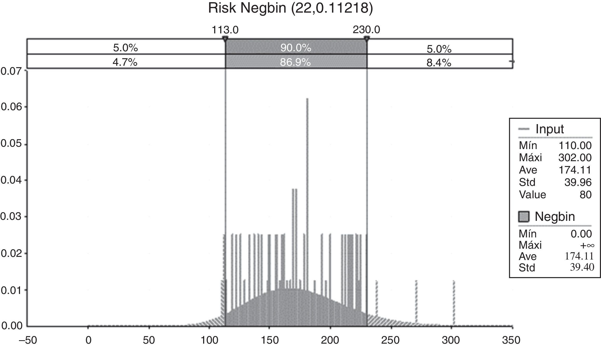
With regard to the probabilities of the labeled node “Pract _Business” (Business Practices), these are associated with events related to actions and activities in the banking sector that generate losses from malpractice and that directly impact the functioning of the banking. In this case, the distribution that best fit the data reported to the ORX is shown in Fig. 3.
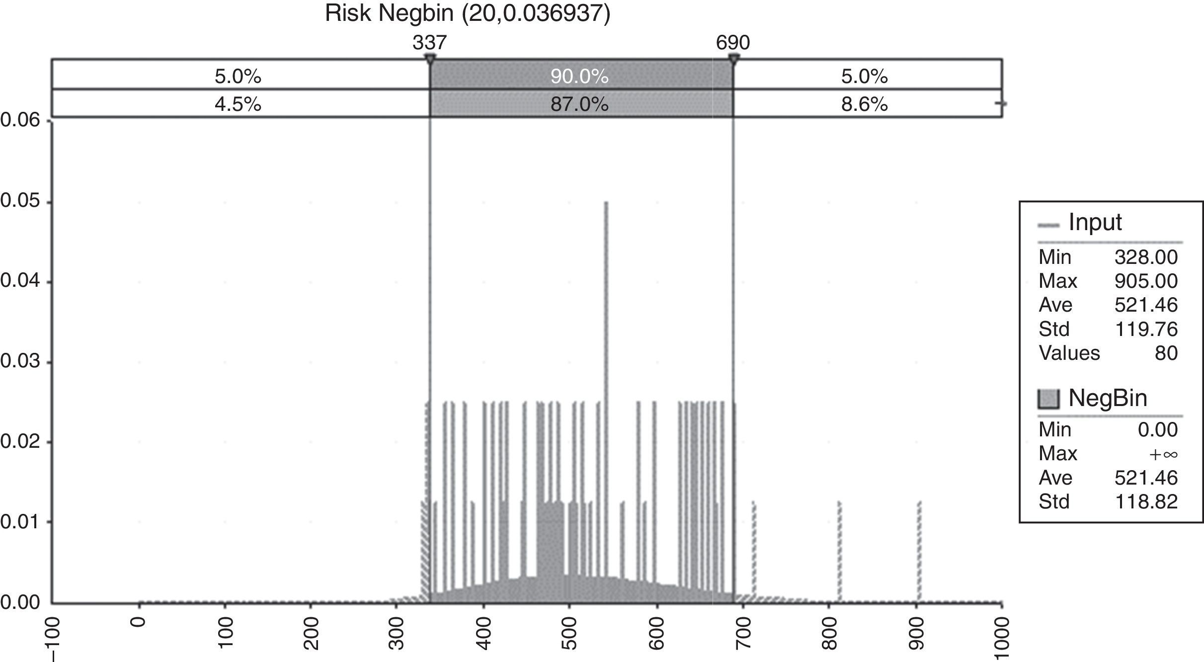
External frauds are exogenous operational risk events for which there is no control but there is a record of their frequency and severity. In this case, the probabilities of occurrence are estimated by fitting a Negative Binomial distribution as shown in Fig. 4.
The proper functioning of banking institutions depends on the performance of their processes. The maturity of these systems is associated with quality management process and product level. The distribution of the node labeled as “Process Management” is shown in Fig. 5.
Finally, for the target node “Frequency”, it is fitted a negative binomial distribution with success probability p=0.012224, an equal number of successes, 20, is assumed. This assumption is consistent with the financial practice and studies of operational risk by assuming that the number of failures usually follows a Poisson or negative Binomial.
- •
Statistical analysis of the severity network
In this section, each node of the severity network is analyzed. For each node with available historical information the distribution that best fit the data is determined. The node “Disaster _TIC” has the following exponential density that best fit the losses caused by failure of not controllable systems and external events. The distribution for disaster and ICT Failure is shown in Fig. 6.
In order to determine the goodness of fit the Akaike's test is used. Moreover, a comparison of theoretical and sample quantiles is shown in Fig. 7.
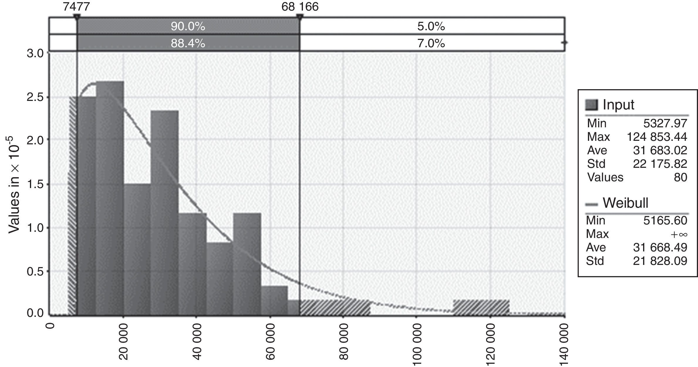
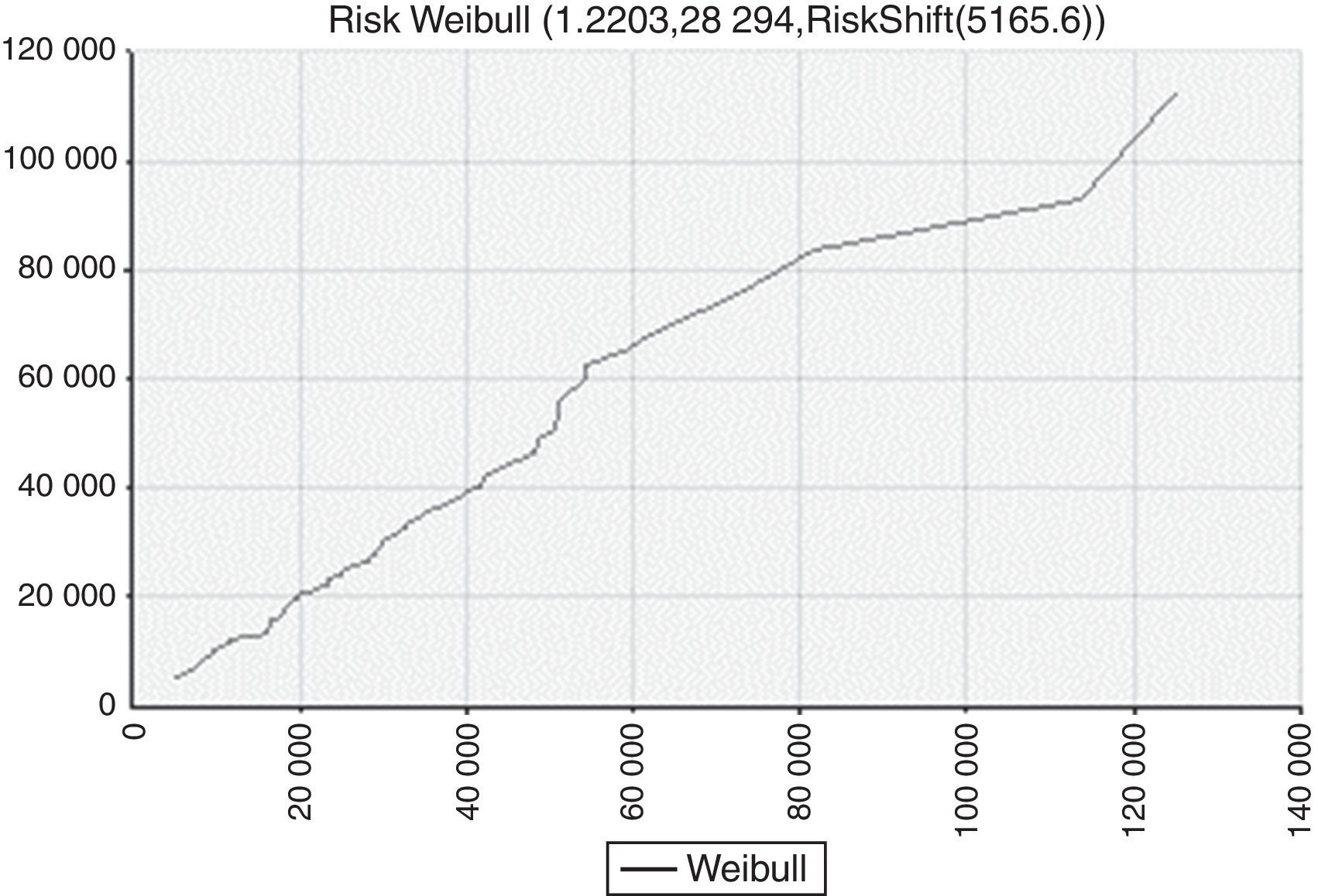
In what follows, a proper fit is seen in most data and information. Thus, the null hypothesis that the sampling distribution is described from a Weibull is accepted. This network node for severity constitutes a prior distribution. Also, for the “People” node the density that best fit available information is an extreme value Weibull density, and it is shown in Fig. 8.
As before, we carry out a test for goodness of fit, and a comparative analysis of quantiles for the theoretical sampling distribution is shown in Fig. 9.
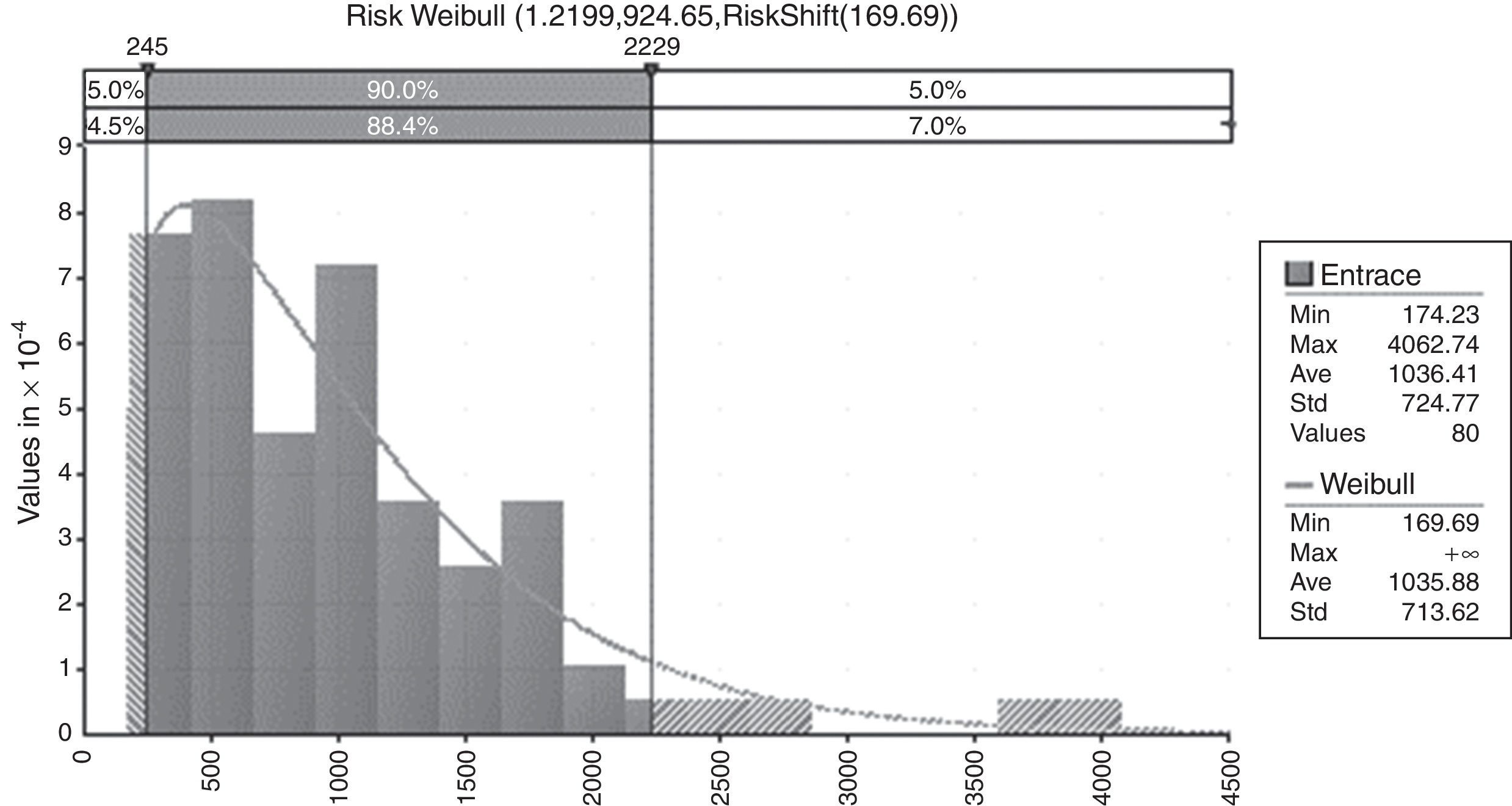
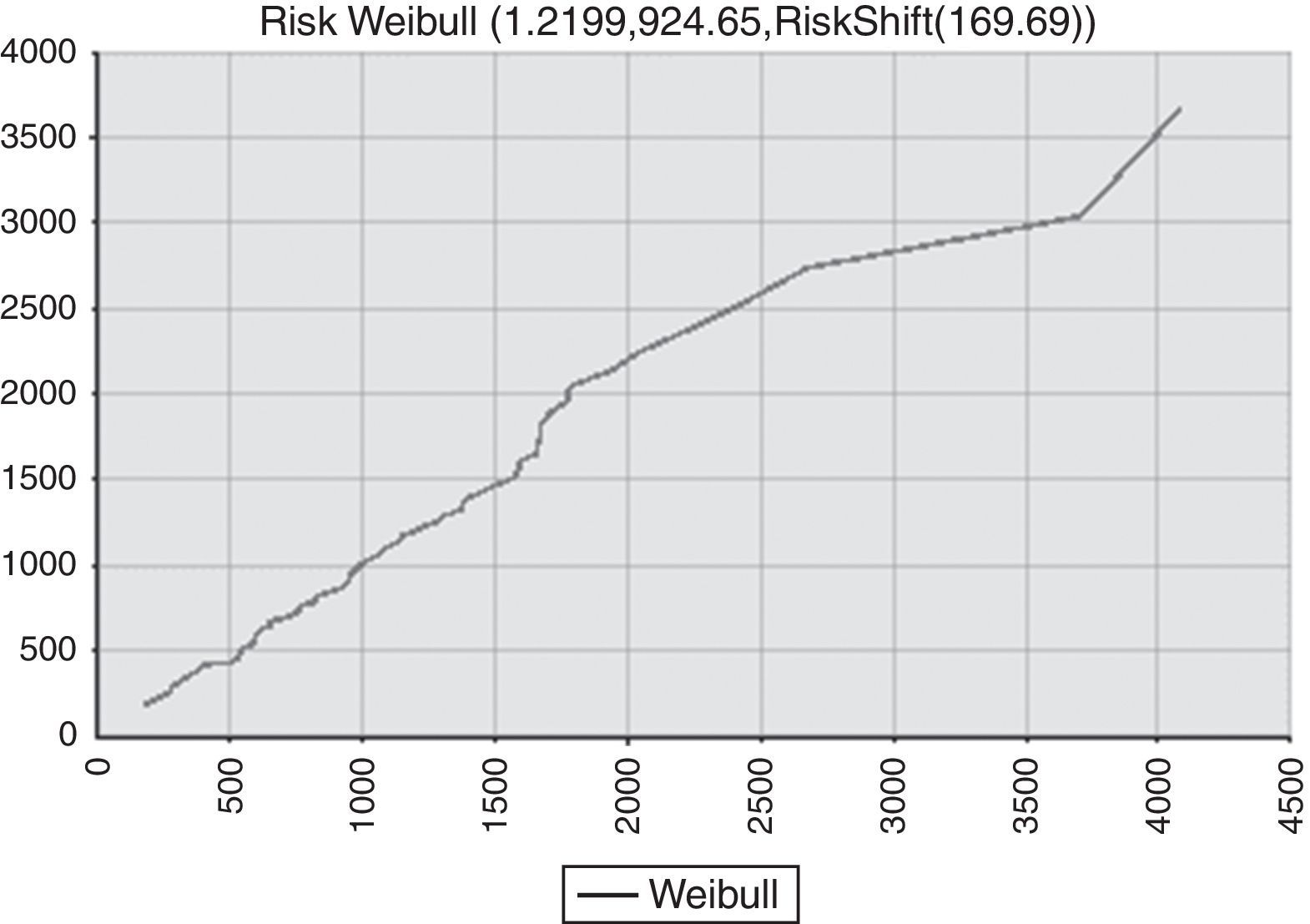
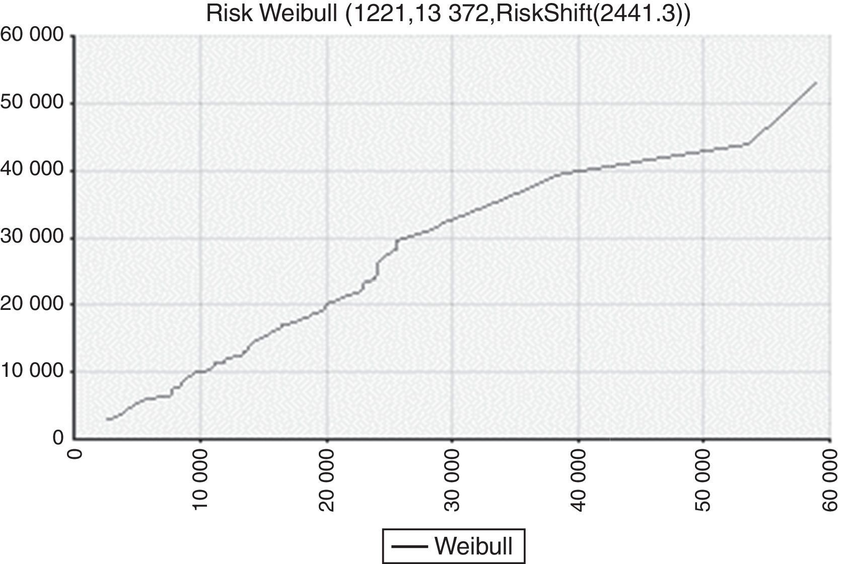
The distribution that best fit the available information for losses caused by events related to the administrative, technical and service processes performed in the various lines of business of the international banking sector is described with an extreme value Weibull distribution as shown in Fig. 10. Also, a comparative analysis of quantiles for the theoretical sampling distribution is shown in Fig. 11.
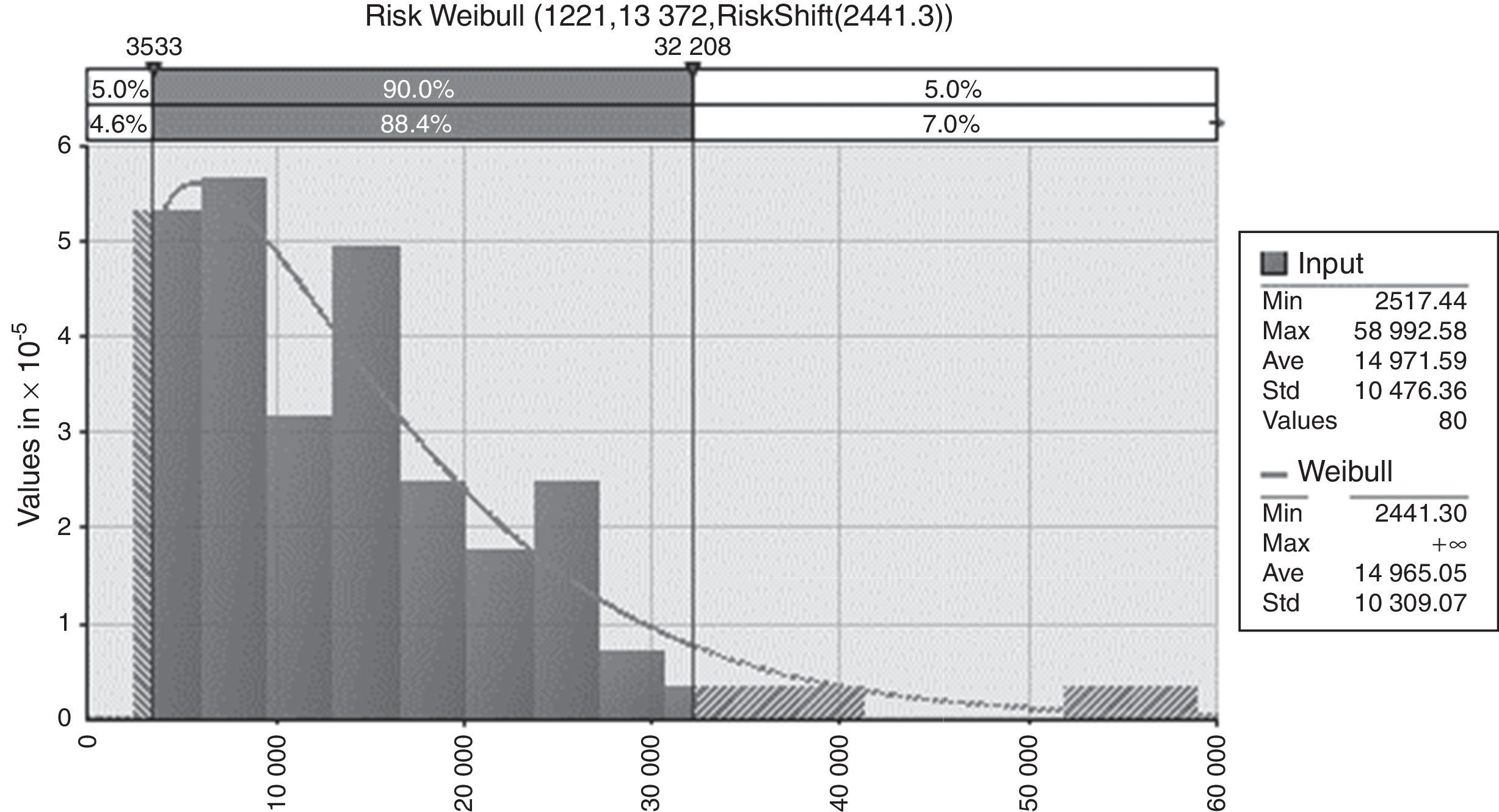
Finally, the target node “Severity” represents the losses associated with the nodes “People”, “Disaster _CIT” and “Processes”. To estimate the parameters of the distribution of severity, a Weibull distribution is adjusted to the severity data. The parameters found are α=1.22 and β=42,592, representing the location and scale, respectively. In the next section, the posterior probabilities will be computed.
- •
The posterior distributions
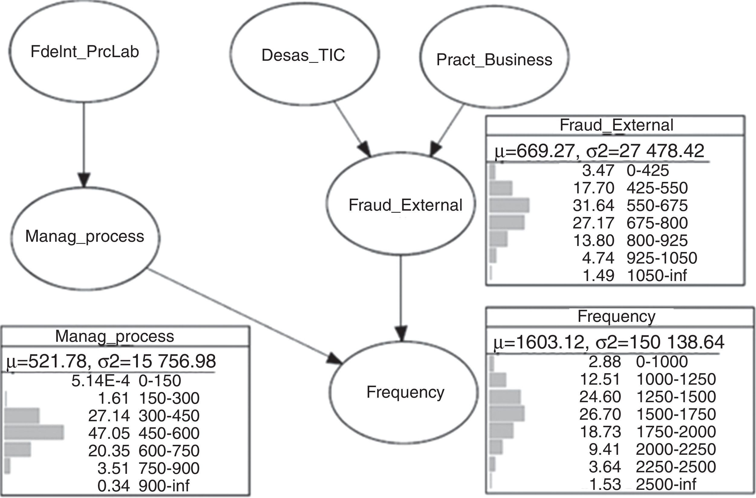
After analyzing each of the networks for frequency and severity, and assigning the corresponding probability distribution functions, the posterior probabilities will be now generated. To do this, inference techniques for the Bayesian Networks will be applied. Particularly, we will be using the junction tree algorithm (Guo & Hsu, 2002). The posterior probabilities for nodes of the network frequency having at least one parent are shown in Fig. 12.
The results of the node “process management” show that there is an approximate 2% chance of failures in a segment considering between 150 and 300 events related to the management process over a period of 20 days; a 27% chance of occurrences in a segment considering between 300 and 450 events; a probability of 0.47 of having failure occurrences in an interval considering between 450 and 600 events, and a 20% chance in a segment considering between 600 and 750 events associated with the administration of banking processes. The calculated probabilities are conditioned by the presence of events related to internal fraud and work processes.
Regarding the node “external fraud” the occurrences between 425 and 550 external frauds over a period of 20 days have an approximate probability of 0.17; between 550 and 675 events a probability of 0.3; between 675 and 800 external fraud the probability is 0.27; and for more than 800 frauds the probability is about 0.2. All these probabilities are conditional on the existence of events related disasters, failures in ICT, and labor practices.
Finally, the probability distribution of the node “Frequency” shows an approximate 15% chance, over a period of 20 days, that failures occur up to 1250; a probability of 25% in a segment considering between 1250 and 1500; a probability of 0.26 in an interval considering between 1500 and 1750 failures; an approximate 19% chance in a segment considering between 1750 and 2000 events; a probability of 0.9 in a segment containing between 2000 and 2250 failures, and approximately 5% chance that 2250 failures occur over a period of 20 days. These are the conditional probabilities to risk factors such as external fraud, process efficiency and people reliability.
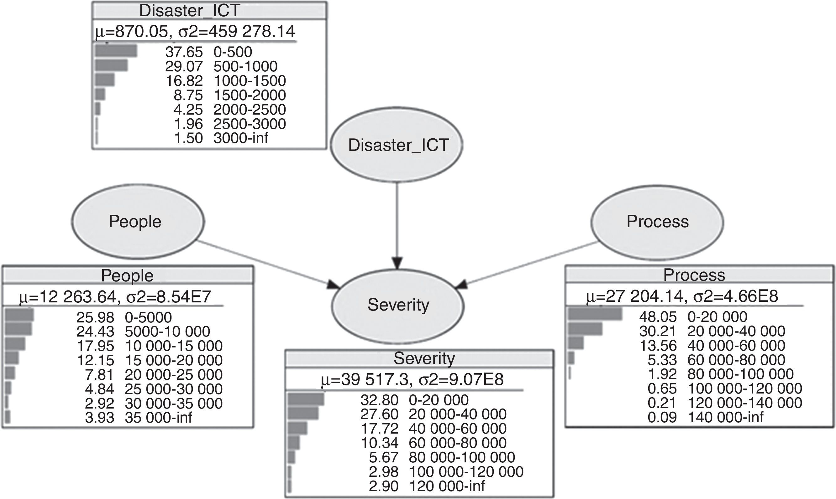
Finally, it is important to point out that for determining the probabilities of each node in the frequency network, the negative binomial plays an important role since there is significant empirical evidence that the frequency of operational risk events have an adequate fit under this distribution. In the case of the network of severity, it has the posterior distribution shown in Fig. 13.
The losses caused by human errors on average are 12,263 Euros in periods of 20 days. With regard to losses for catastrophic events such as demonstrations, floods, and ICT failure, among others, are on average 870 Euros. In terms of process failures on average they have a loss every 20 days of 27,204 Euros. The probability distribution of the node “Severity” shows that there is a probability of 0.33 of the occurrence of a loss between 0 and 20,000 Euros; a probability of 0.2 between 20,000 and 40,000, a 10% chance between 60,000 and 80,000 Euros, a 6% chance between 80,000 and 100,000 Euros, and approximately a 6% chance that the loss be greater than 100,000 Euros in a period of 20 days.


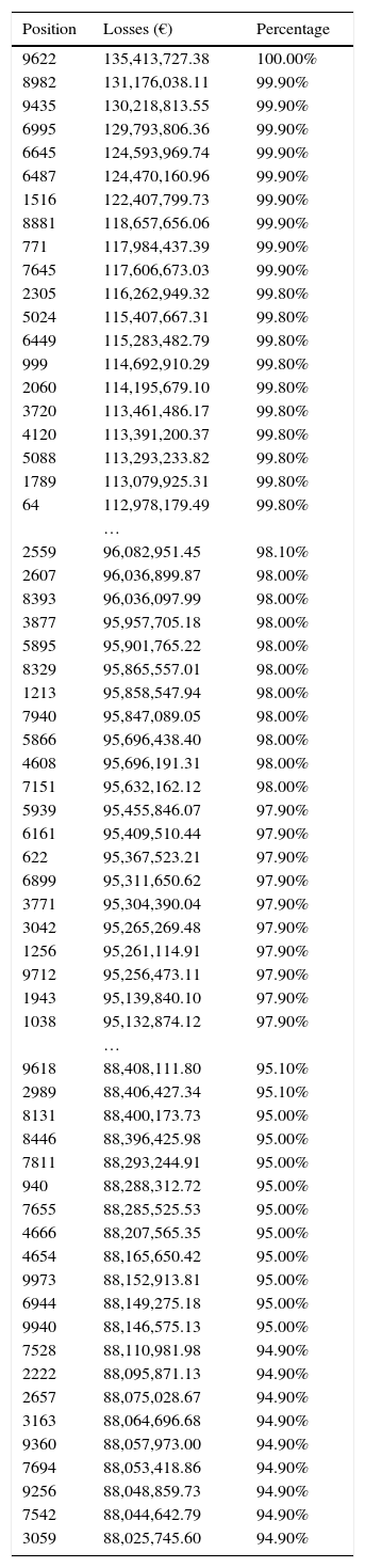
Once we have carried out the Bayesian inference process to obtain posterior distributions for the frequency of OR events and the severity of losses in the previous section, we now proceed to integrate both distributions through Monte Carlo8 simulation by using the “Compound” function of @Risk. To achieve this goal, we generate the distribution function of potential losses by using a negative binomial for frequency and an extreme value Weibull distribution for severity.9 It is worthy to mention that Monte Carlo simulation method has the disadvantage that it requires high processing capacity and, of course, is based on a random number generator. For the calculation of OpVar the values obtained are arranged for expected losses in descending order and the corresponding percentiles are calculated in Table 3. Accordingly, if we calculate the OpVaR with a confidence level of 95%, we have a maximum expected loss of €88.4 million over a period of 20 days for the group of international banks associated to the ORX.10
Percentiles for Bayesian model.
| Position | Losses (€) | Percentage |
|---|---|---|
| 9622 | 135,413,727.38 | 100.00% |
| 8982 | 131,176,038.11 | 99.90% |
| 9435 | 130,218,813.55 | 99.90% |
| 6995 | 129,793,806.36 | 99.90% |
| 6645 | 124,593,969.74 | 99.90% |
| 6487 | 124,470,160.96 | 99.90% |
| 1516 | 122,407,799.73 | 99.90% |
| 8881 | 118,657,656.06 | 99.90% |
| 771 | 117,984,437.39 | 99.90% |
| 7645 | 117,606,673.03 | 99.90% |
| 2305 | 116,262,949.32 | 99.80% |
| 5024 | 115,407,667.31 | 99.80% |
| 6449 | 115,283,482.79 | 99.80% |
| 999 | 114,692,910.29 | 99.80% |
| 2060 | 114,195,679.10 | 99.80% |
| 3720 | 113,461,486.17 | 99.80% |
| 4120 | 113,391,200.37 | 99.80% |
| 5088 | 113,293,233.82 | 99.80% |
| 1789 | 113,079,925.31 | 99.80% |
| 64 | 112,978,179.49 | 99.80% |
| … | ||
| 2559 | 96,082,951.45 | 98.10% |
| 2607 | 96,036,899.87 | 98.00% |
| 8393 | 96,036,097.99 | 98.00% |
| 3877 | 95,957,705.18 | 98.00% |
| 5895 | 95,901,765.22 | 98.00% |
| 8329 | 95,865,557.01 | 98.00% |
| 1213 | 95,858,547.94 | 98.00% |
| 7940 | 95,847,089.05 | 98.00% |
| 5866 | 95,696,438.40 | 98.00% |
| 4608 | 95,696,191.31 | 98.00% |
| 7151 | 95,632,162.12 | 98.00% |
| 5939 | 95,455,846.07 | 97.90% |
| 6161 | 95,409,510.44 | 97.90% |
| 622 | 95,367,523.21 | 97.90% |
| 6899 | 95,311,650.62 | 97.90% |
| 3771 | 95,304,390.04 | 97.90% |
| 3042 | 95,265,269.48 | 97.90% |
| 1256 | 95,261,114.91 | 97.90% |
| 9712 | 95,256,473.11 | 97.90% |
| 1943 | 95,139,840.10 | 97.90% |
| 1038 | 95,132,874.12 | 97.90% |
| … | ||
| 9618 | 88,408,111.80 | 95.10% |
| 2989 | 88,406,427.34 | 95.10% |
| 8131 | 88,400,173.73 | 95.00% |
| 8446 | 88,396,425.98 | 95.00% |
| 7811 | 88,293,244.91 | 95.00% |
| 940 | 88,288,312.72 | 95.00% |
| 7655 | 88,285,525.53 | 95.00% |
| 4666 | 88,207,565.35 | 95.00% |
| 4654 | 88,165,650.42 | 95.00% |
| 9973 | 88,152,913.81 | 95.00% |
| 6944 | 88,149,275.18 | 95.00% |
| 9940 | 88,146,575.13 | 95.00% |
| 7528 | 88,110,981.98 | 94.90% |
| 2222 | 88,095,871.13 | 94.90% |
| 2657 | 88,075,028.67 | 94.90% |
| 3163 | 88,064,696.68 | 94.90% |
| 9360 | 88,057,973.00 | 94.90% |
| 7694 | 88,053,418.86 | 94.90% |
| 9256 | 88,048,859.73 | 94.90% |
| 7542 | 88,044,642.79 | 94.90% |
| 3059 | 88,025,745.60 | 94.90% |
Source: Own elaboration.
Transnational banks generate large amounts of information from the interaction with customers, with the industry and with internal processes. However, the interaction with the individuals involved in the processes and systems also required some attention and this considered by the Operational Riskdata eXchange Association that has stated several standards for the registration and measurement of operational risk.
This paper has provided the theoretical elements and practical guidance necessary to identify, quantify and manage OR in the international banking sector under the Bayesian approach. This research uses elements more attached to reality such as: specific probability distributions (discrete or continuous) for each risk factor, additional data and information updating the model, and relationships (causality) of risk factors. It was shown that the BN framework is a viable option for managing OR in an environment of uncertainty and scarce information or with questionable quality. The capital requirement is calculated by combining statistical data with opinions and judgments of experts, as well as, external information, which is more consistent with reality. The BNs as a tool for managing OR in lines of business of the international banking sector have several advantages over other models:
- •
The BN is able to incorporate the four essential elements of Advanced Measurement Approach (AMA): internal data, external data, scenario analysis and factors reflecting the business environment and the control system in a simple model.
- •
The BN can be built into a “multi-level” model, which can display various levels of dependency between the various risk factors.
- •
The BN running on a network of decision can provide a cost-benefit analysis of risk factors, where the optimum controls are determined within a scenario analysis.
- •
The BN is a direct representation of the real world, not a way of thinking as neural networks. Arrows or arcs in networks stand for the actual causal connections.
It is important to point out that the CVaR used in the Bayesian approach is consistent in the sense of Artzner et al. (1999), but also summarizes the complex causal relationships between the different risk factors that result in operational risk events. In short, because the reality is much more complex than independent events identically distributed, the Bayesian approach is an alternative to model a complex and dynamic reality.
Finally, among the main empirical results, it is worth mentioning that after calculating the OpVaR, with a confidence level of 95%, the maximum expected loss over a period of 20 days for the group of international banks associated to the ORX was €88.4 million, which is a significant amount to be considered to manage operational risk in ORX for the studied lines of business of commercial banks.
Conflict of interestsThe authors declare no conflict of interest.
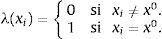
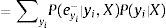
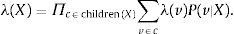
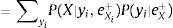
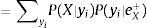
Among the accurate inference algorithms, we have: Pearl's (1988) polytree; Lauritzen and Spiegelhalter (1988) clique tree, and Cowell, Dawid, Lauritzen, and Spiegelhalter's (1999) junction tree. Pearl's method is one of the earliest and most widely used. The spread of beliefs according to Pearl (1988) follow the following process. Let e be the set of values for all observed variables. For any variable X, e can be divided into two subsets: eX− representing all the observed variables descending from X, and eX+ corresponding to all other observed variables. The impact of the observed variables on the beliefs of X can be represented by the following two values:
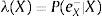
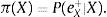
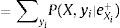
That is, λ(X) and π(X) are vectors whose elements are associated with the values of X:


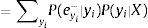
The posterior distribution is obtained by using (A1) and (A2), thus
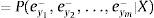
where α=1/P(e). In order to infer new beliefs, Eq. (A5) is used. The values of λ(X) and π(X) are calculated as follows: λ(Y1,Y2,…,Ym) where Y1,Y2,…,Ym are children of X. When X takes the value x0, the elements of vector λ(X) are assigned as follows: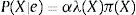
In the case in which X has no value, we have eX−=⋃i=1meyi−. Hence, by using (A1), λ(X) expands as:


By using the fact that ey1−,ey2−,…,eym− are conditionally independent, and defining
it follows that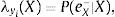
The last expression shows that in calculating the value of λ(X) the values of λ and conditional probabilities of all children X are required. Therefore, vector λ(X) is calculated as:
For the calculation of π(X) it is used the father Y of the X values. Indeed, by using (A2), it follows
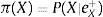
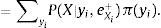
This shows that when calculating π(X), the values of π of the fathers X and their conditional probabilities are necessary.
There might be some difficulties in dealing with Pearl's inference method due to the generated cycles when the directionality is eliminated. Cowell et al. (1999) junction tree algorithm may overcome this situation. First, it converts a directed graph into a tree whose nodes are closed to proceed to spread the values of λ and π through the tree. The summarized procedure is as follows:
- 1.
“Moralize” the BN.
- 2.
Triangulate the moralized graph.
- 3.
Let the cliques of the triangulated graph be the nodes of a tree, which is the desired junction-tree.
- 4.
Propagate λ and π values throughout the junction-tree to make inference. Propagation will produce posterior probabilities.
When referring to experts, they are banking officials who have the experience and knowledge of the operation and management of the bank business lines.
Usually, to measure the maximum expected loss (or economic capital) by OR value it is used the Conditional Value at Risk (CVaR).
For a complete analysis on the non coherence of VaR see Venegas-Martínez (2006).
For a review of issues associated with Bayes’ theorem see Zellner (1971).
These questions are a very important topic Bayesian inference; see, in this regard, Ferguson (1973).
The following definitions will be needed for the subsequent development of this research: Definition 1, Bayesian networks are directed acyclic graph (DAGs); Definition 2, a graph is defined as a set of nodes connected by arcs; Definition 3, if between each pair of nodes there is a precedence relationship represented by arcs, then the graph is directed; Definition 4, A cycle is a path that starts and ends at the same node; and Definition 5, A path is a series of contiguous nodes connected by directed arcs.
See Jensen (1996) for a review of the BN theory.
The simulation results are available via e-mail request marzan67@gmail.com.
- Transferibilidad de competencias profesionales, impactos y estrategias en 2 estudios de caso en la frontera norte de México
- Colectivos de inversión empresarial: una opción hacia el desarrollo local 1 , 2
- Governance codes: facts or fictions? a study of governance codes in colombia 1 , 2
- La influencia del desempeño social corporativo en la satisfacción laboral de los empleados: una revisión teórica desde una perspectiva multinivel 1 , 2

www.publicationethics.org.
