


Since 2000, Cali has had the highest mean annual homicide rate among the major Colombian cities. The model of Mills (1972) is extended to include the homicide per commune (from 2005 to 2012) as a measure of social distance, and to quantify the effect of this phenomenon on land prices (mean appraisals). Using an annual panel, the estimates of the model – the family violence rate being the instrumental variable – show that an increase in the homicide rate of one unit reduces the appraisals by 1.6%. One plausible interpretation is that homicides operate as a regressive tax on property wealth in Cali because it is more concentrated in the communes of the lower socio-economic stratum, systematically expanding the intra-urban social distance.
Desde el año 2000 Cali tuvo la tasa promedio anual de homicidio más alta entre las principales ciudades colombianas. Nosotros ampliamos el modelo de Mills (1972), incluyendo el homicidio por comunas (durante 2005-2012) como medida de distancia social, para cuantificar el efecto de este fenómeno sobre los precios de la tierra (avalúos medios). Empleando datos panel, las estimaciones del modelo — usando la violencia familiar como variable instrumental — evidencian que un crecimiento unitario de la tasa de homicidio reduce los avalúos hasta en un 1,6%. Una interpretación plausible es que el homicidio opera como un impuesto regresivo sobre la riqueza inmueble, pues en Cali se concentra más en las comunas de menor estrato socioeconómico, ampliando sistemáticamente la distancia social intraurbana.
The economic literature has been interested in measuring the implications of homicide due to its possible impact on countries’ aggregate performance. However, when the event occurs near a house or real property, beyond generating a possible emotional effect, it may have effects on the microeconomic scale that can be quantified. This paper aims to reveal the magnitude of these effects on variables such as the wealth of individuals and, in particular, the value of the essential property, namely land. Moreover, the paper constitutes an important element in the discussion of optimal applications of traditional policies against crime.
The mechanism for this kind of study that has prevailed in the economic literature is the estimation of hedonic price models. However, due to obvious limitations regarding the data volume for this paper, here we present the use of one extended version of the model proposed by Mills (1972). An advantage of this model is that it enables us to observe the spatial urban performance of land prices through friction (negative effect) generated by the physical distance with respect to the city center (hereinafter DCC). The other advantage of extending the model is that it allows us to add homicide as another friction element but concerning the social distance.1
This sociological concept is relevant because its variability may be an element that exacerbates aggression and criminal behavior (Arteaga and Lara, 2004). This argument, seen otherwise, means that in areas with higher homicide rates – which could be those that are the poorest or have a lower life quality – vicious circles and a self-sustained extension of social distance could be created that could exert a negative impact on land prices, generating an adverse effect on the wealth of individuals or households and thus impoverishing them more.
Considering that the city of Cali (Colombia) has presented relatively stable homicide rates during this century – higher rates than those of other major cities in the country, of which the location seems to result in inertial performance in some areas – we estimate the magnitude of the homicide effect on land prices, approximated by mean appraisals of the plot of land per commune (hereinafter MAPC). The data come from a panel built for 22 communes of the city between 2005 and 2012, obtained from public sources, which includes interest variables and some controls that quantify amenities and economic cycle changes. It is important to emphasize that this panel is the most complete and reliable one that is publicly available for the city, although it generates restrictions by the non-inclusion of more periods of time or variables that are considered in similar research.
Given the model structure chosen and the possibility of simultaneity between the homicide rate and the land price, the first set of estimates was made following the ordinary least square method (hereinafter OLS) with the Hausman endogeneity test (1978). However, to give more robustness to the exercises, a second set of estimates was produced using least squares in two stages (hereinafter 2SLS) with the family violence rate as the instrumental variable.
Among the most important results of the two sets of estimates, we found that: (i) there is evidence that the city does not have a monocentric urban structure, (ii) no endogeneity exists between the homicide rate and the land price and (iii), most importantly, according to the OLS estimates, there is evidence that when the homicide rate rises by one unit, the MAPC is reduced by a value that oscillates between 0.5 and 1.1% under the estimated model; in addition, the range of values can reach 1.66 percentage points based on the results of the 2SLS estimates. This shows that the homicide rate generates a significant negative wealth effect on individuals, which could be interpreted as a regressive tax because it has a proportional impact on the wealth of the poorest – the lowest stratum – and reasonably can be assumed to be a factor that expands the social distance between the city communes.
From this we infer that the homicide rate impoverishes the poorest people systematically. This derivation reiterates the importance of improving the management efficiency of the anti-homicide public policy as well as the care that the government and research agencies should take to disseminate ciphers about this kind of crime. To achieve this result, the paper is organized as follows: In Section 2, we describe some stylized facts about the phenomenon in Cali. In Section 3 we discuss some previous works available in the literature. In Sections 4–6, we lay out the theoretical and methodological specifications of our analysis. In Sections 7 and 8, we present the empirical results. Finally, in Section 9, we present our main conclusions.
2Some stylized factsFollowing the UNODC (2014), the top five of the countries in the global context with the highest average homicide rate between 2000 and 2012 are Honduras (62.5 homicides per 100,000 inhabitants), followed by El Salvador (52.1), Jamaica (48.8), Colombia (44.4) and Venezuela (43.2). However, according to the Vice President of the Republic of Colombia, Cali exceeds these measurements, reaching an average of 79. This situation involves dramatic differences, because, in the same period, the city presented the highest rate among the 13 major cities in Colombia,2 followed by Medellin (78.8), Pereira (76) and Cucuta (75), but with the aggravating factor that in these cities the rate's variability was greater3 and followed a downward trend, while in Cali the rate remained stable. For example, in Medellin the average rate variance was −4.34%, while in Cali it was only −0.8%.
Although it is not the focus of this work, it is convenient to mention that this scenario is attributed, among other things, to the influence of drug trafficking and crime, the widespread use of firearms as a victimizing mechanism and the stability in the localization of a large number of murders in the areas or communities with the poorest life quality indicators (Concha et al., 2002; Observatorio Social de Cali, 2011; Loaiza, 2012; Escobedo, 2013).
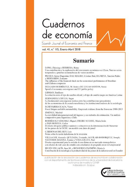
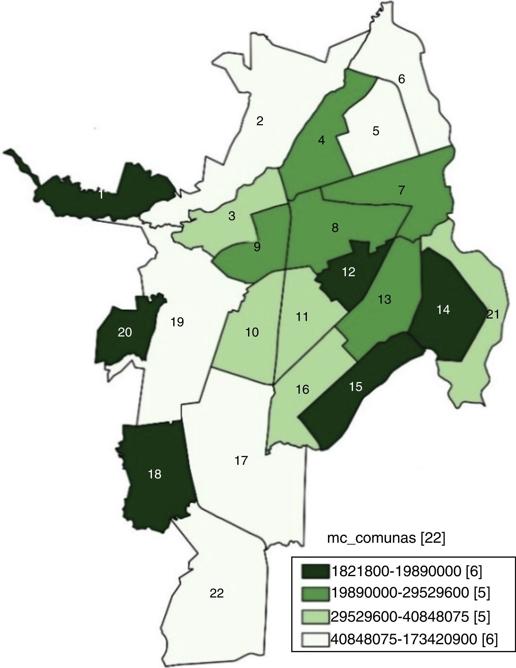
Therefore, it is plausible that a serious phenomenon has an impact on the real wealth of individuals. In the case of Cali, the possible relationship between the homicide rate and the value of real property has not been studied so far, except for parts of Delgado's (2012) work and some descriptive evidence. For example, the overall view shown in Figs. 1 and 2 warns of an inverse association between the MAPC and the homicide rate in 2012.
 2012.")
.")
It is necessary to be aware that, while the highest homicide rates are concentrated in eastern and western hillside communes (excluding commune 1) accompanied by a comparatively lower appraisal,4 the opposite happens in the communes with a higher appraisal (except commune 22) that share lower homicide rates, placed in parallel to the fifth and tenth streets, the main longitudinal streets of the city. Likewise, an intermediate group of communes – including commune 3, where the DCC is located – involves similar quartiles for homicide and appraisal on the two maps, considering that these are presented inverted.
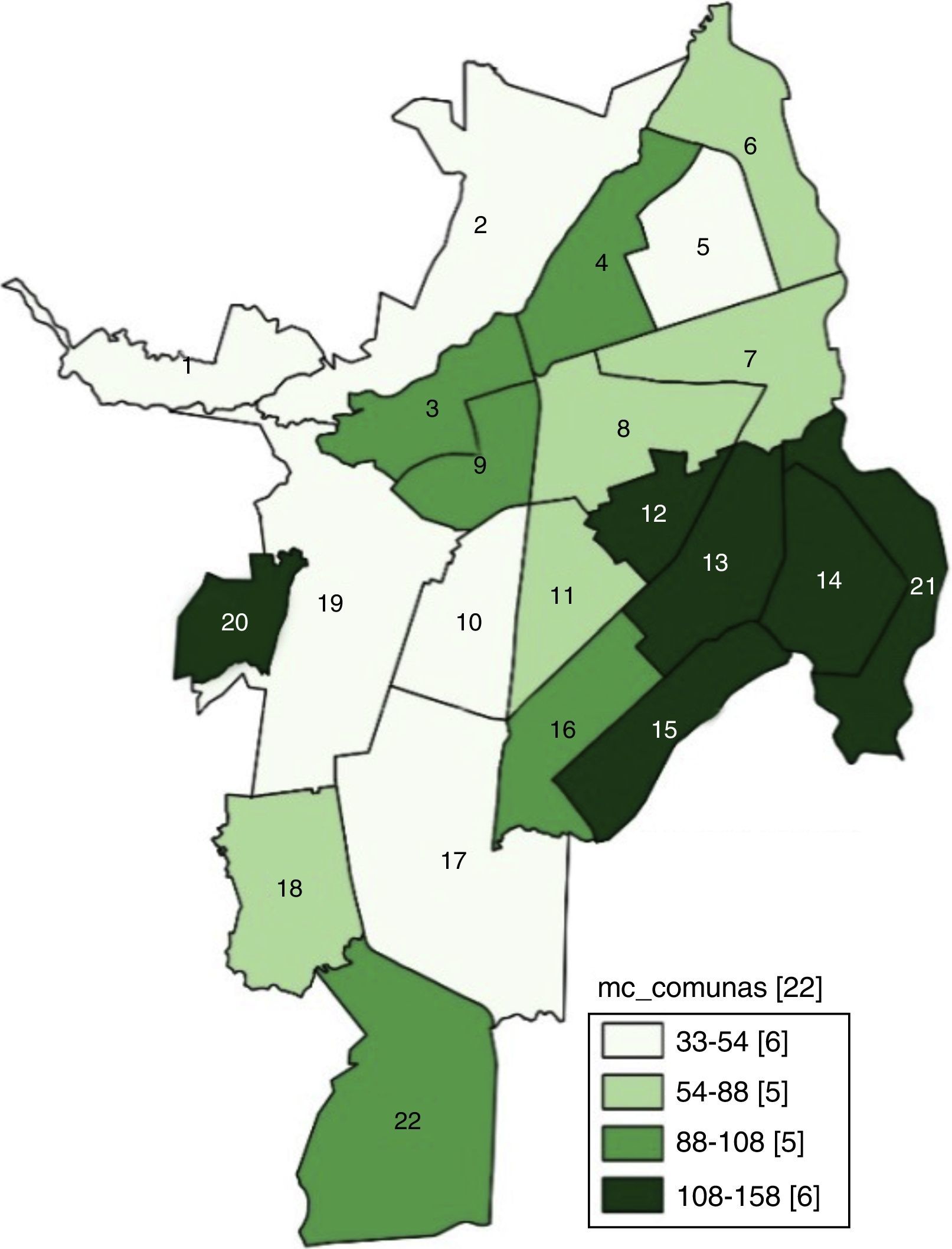
In addition, Fig. 3 shows that the inverse correlation between the variables – in both cases measured as the average over the period 2005–2012 – can be considered as a stylized fact. Despite the time period not being sufficiently large to analyze more structural dynamics as a proxy for land prices, some inertia may be noticed in them as well as in the homicide rate.
3Background
This article contributes to the extensive literature on the effects of crime on the value of real property and mostly assumes endogeneity (by simultaneity) between these variables, focusing on OLS and 2SLS estimates (with instrumental variables). Many studies have used hedonic pricing models to determine individuals’ willingness to pay to avoid the effects of crime on the price of their assets.
For example, Buonanno et al. (2012) analyzed the real estate market data and a victimization survey for Barcelona between 2004 and 2006; the authors estimated that the crime perception affects negatively the property prices. In addition to crime, Troy and Grove (2008) included the variable “live near a park,” showing that, in the case of Baltimore in 2004, the effect of that variable is positive as long as the park has lower rates of rape and robbery.
Meanwhile, Pontes et al. (2011) estimated the cost of crime implicit in the prices of the residences of Belo Horizonte in 2004 with the aim of capturing individuals’ willingness to pay to live in safer areas. Their most important discovery was that robberies of passers-by affect the price of properties in a greater proportion than homicides, because the former occur more frequently. In addition, Gaviria et al. (2008) found that Bogota's households in higher socioeconomic strata pay more for their property to avoid an increase in homicide rates. To achieve this, they used data from the 2003 Survey of Life Quality. A similar exercise was carried out by Bishop and Murphy (2011) through the estimation of a dynamic demand model that showed that, for the period 1990–2008, California Bay households were willing to pay US$472 on average per year to avoid a 10% increase in the crime rate.
On the other hand, the use of instrumental variables allowed Pope and Pope (2012) to find an inverse relationship between the presence of crime and the property values in the cases of twelve states and five metropolitan areas in the United States during the 1990s. A similar result was obtained by Ihlanfeldt and Mayock (2010) from a panel composed of information on tax and criminal incidents in Miami-Dade County properties between 1999 and 2007. Using commercial land use variables as instruments revealed that the crime density explains the variation in the housing price index and that aggravated theft is the crime that has the most negative effects.
Impact assessment has also been used as a tool to study this research topic, in particular with the differences-in-differences method. In the case of Rio de Janeiro, Frischtak and Mandel (2012) analyzed the impact of the system of police stations in low-income areas on crime and real estate prices. The exercises, conducted with data from 2008 to 2011, showed that new stations produce a substantial and positive effect on property prices but a negative one on certain crimes; they also showed that the historical crime rate has persistent effects on real estate values.
Likewise, Klimova and Lee (2014) measured the impact of the occurrence of homicides on property prices and their rents in Sydney. The researchers found that real estate values were reduced by almost 4% for properties – with similar features – located some distance from the venue. However, they found no effect of the homicides on rental prices.
On the other hand, this article also contributes to the broad local literature that has studied homicide in Cali city. Many of these studies were based on descriptive analysis, especially those undertaken since the 1990s (Concha et al., 2002; Observatorio Social de Cali, 2011; Loaiza, 2012; Escobedo, 2013), highlighting the influence of drug trafficking on the criminal and murderous dynamics, the widespread use of firearms as a victimizing element, the stable decreasing tendency of data from other cities, like Bogota and Medellin, and inertia in the high-density locations of homicide.
Given the above, another line of research has analyzed the phenomenon from the geographical point of view; for example, Ortiz (2010) characterized the neighborhoods with a high concentration of homicides, asserting that they have a lower life quality, measured by indicators of unsatisfied basic needs. However, he added that another factor that has an impact on a major criminal presence is the location of massive and poorly regulated economic activities affecting the urban environment, such as marketplaces and recreation and leisure sites. Meanwhile, Loaiza (2012) found that western and eastern slope areas adjacent to the Cauca River have a higher probability of homicide and included this in calculating the homicide propensity index per commune.
Inferential statistics has also been used to study the issue; based on this methodology, Vásquez (2010) found a positive association between unemployment and crime and then related the economic situation to the possibility of being a victim of theft or murder, concluding that a crisis situation can lead to a greater likelihood of homicide. At the same time, using a Poisson regression, Arango et al. (2009) estimated that men aged between 20 and 30 years have a greater relative risk of being killed and that guns are the most common weapon used by victimizers. Furthermore, Díaz and Graffe (2014) discovered using fixed-effect estimates that variables such as the education access rate, cultural service coverage and security service coverage are significant in explaining the homicide rate in Cali per commune between 2002 and 2012.
Finally, this paper contributes to the sparse local literature that relates crime to land prices. In that sense, Delgado (2012) used a panel for the period 2000–2010 to demonstrate that overcrowding, preferential service coverage and population age composition – the majority being between 16 and 24 years old – are significant in explaining the homicide rate in the city; however, he included the mean appraisal of properties as a control variable. According to his estimates, an increase of 1 million COP in this variable reduces the homicide rate by 0.16. Nevertheless, Delgado's work (2012), unlike the present paper, did not consider the possible simultaneity between these variables – the endogeneity source – that would prevent the estimates, as above, from being biased and over- or underestimating the parameter for appraisals.
4The modelMills (1972) described the urban spatial performance of land prices and predicted that there is an inverse relationship between land prices and distance from the main center (DCC) that could be represented by a decreasing exponential function. The theoretical foundation of this relationship is that the highest land prices in cities are in the DCC, because the economic activities that attract households and firms are concentrated in the DCC. This model is part of the family of seminal space economy models proposed by Von Thünen.5 Mathematically, the model is written in the following way:
where Pi is the plot of land price i, EXP(β0) is the mean land price in the DCC and β1<0 is the price–distance gradient, which measures the decline grade in the land price while the plot of land i moves away from the DCC at a distance Di.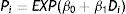
Expression (1) describes a monocentric city structure; however, this system may be weakened if the land price in the DCC is reduced below that of other areas, which could be due, among many factors that will not be investigated in depth here, to the rise of new and improved commercial sites inside these areas and/or to the search by households located in residential areas with a lower population density. To predict this situation, we propose an extension model as follows:

Given (2), if β2>0, the city would not be monocentric, because from a certain plot of land i the land prices may be incremented by a greater distance from the DCC.
On the other hand, in relation to the distance, although it is logical in a spatial economy context to measure it in physical units and accessibility to the DCC, underlying this concept is the fact that it can be analyzed as a friction factor on land prices, which opens up the possibility to measure the distance through variables that also reflect friction as a social distance or, conversely, reduce it with amenities. Accordingly, the model can be formulated thus:

For (3) it would be expected that β3<0 and β4>0.6 These signs may be explained as follows: in relation to amenities (θ), they are factors that increase the welfare of landowners and, by definition, improve their market value. Among them, Gaviria et al. (2008) included access and quality of public goods and services (roads, parks and green areas, transport and security, among others).
Regarding social distance (H), in the concept of sociological studies, it is important to consider the main idea for this research, which is reflected by criminal behavior and conflict, in our case by the homicide rate per area. As all the distances in the model, it is a friction mechanism on land prices with the difference that if the wealth and consequently the life quality are reduced, it could replicate itself, generating a trap exerting adverse effects on the real property value.
5DataThe data were taken from the Cali en Cifras documents for the period 2005–2012, and the spatial units are the 22 communes of the city. Government agencies such as Metro Cali S.A. and DAGMA (Administrative Department of Environmental Management, with its acronym in Spanish) were consulted as well. This allowed us to build panel data consisting of 176 observations.7 The land prices were approximated by the MAPC deflated by the 2008 prices. The homicide rate and family violence rate (reported cases) were calculated per 100,000 habitants. Other variables used for each commune were: physical distance from the DCC, stratum mode as an income proxy variable and, as amenities, banks, malls with cinemas, marketplaces, a public transport station system (MIO) and large parks (see Appendix 1).
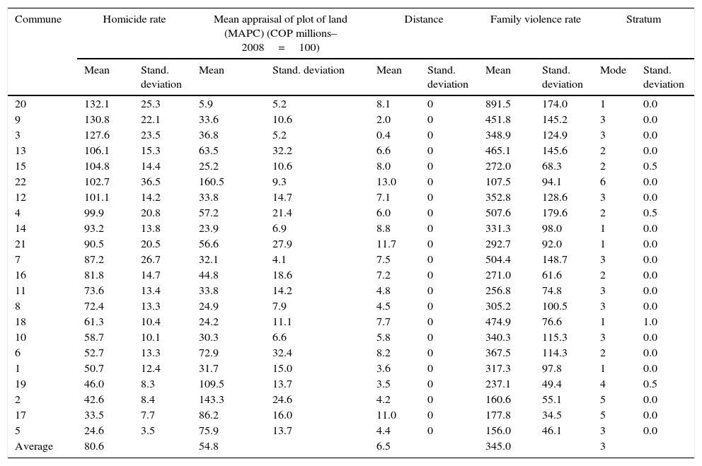
Table 1 shows some characteristics of the variables. It can be seen that the 5 communes – including commune 3, where the DCC is located – that present the highest mean homicide rates have strata between 1 and 3, contrary to the 5 communes that show lower values. This reinforces the importance of the social distance concept to the explanation of the criminal phenomenon. On the other hand, it is noteworthy that both commune 2 and commune 19 are bordered by communes with a lower stratum and mean appraisal, such as communes 1 and 20 (see Figs. 1 and 2). This shows that the socio-economic configuration of the city in that area is not monotonous and presents a polarization or rupture that is more evident when looking at commune 20, which has the steepest mean both in family violence and in homicide, in conjunction with the lowest appraisals.
Descriptive statistics.
| Commune | Homicide rate | Mean appraisal of plot of land (MAPC) (COP millions–2008=100) | Distance | Family violence rate | Stratum | |||||
|---|---|---|---|---|---|---|---|---|---|---|
| Mean | Stand. deviation | Mean | Stand. deviation | Mean | Stand. deviation | Mean | Stand. deviation | Mode | Stand. deviation | |
| 20 | 132.1 | 25.3 | 5.9 | 5.2 | 8.1 | 0 | 891.5 | 174.0 | 1 | 0.0 |
| 9 | 130.8 | 22.1 | 33.6 | 10.6 | 2.0 | 0 | 451.8 | 145.2 | 3 | 0.0 |
| 3 | 127.6 | 23.5 | 36.8 | 5.2 | 0.4 | 0 | 348.9 | 124.9 | 3 | 0.0 |
| 13 | 106.1 | 15.3 | 63.5 | 32.2 | 6.6 | 0 | 465.1 | 145.6 | 2 | 0.0 |
| 15 | 104.8 | 14.4 | 25.2 | 10.6 | 8.0 | 0 | 272.0 | 68.3 | 2 | 0.5 |
| 22 | 102.7 | 36.5 | 160.5 | 9.3 | 13.0 | 0 | 107.5 | 94.1 | 6 | 0.0 |
| 12 | 101.1 | 14.2 | 33.8 | 14.7 | 7.1 | 0 | 352.8 | 128.6 | 3 | 0.0 |
| 4 | 99.9 | 20.8 | 57.2 | 21.4 | 6.0 | 0 | 507.6 | 179.6 | 2 | 0.5 |
| 14 | 93.2 | 13.8 | 23.9 | 6.9 | 8.8 | 0 | 331.3 | 98.0 | 1 | 0.0 |
| 21 | 90.5 | 20.5 | 56.6 | 27.9 | 11.7 | 0 | 292.7 | 92.0 | 1 | 0.0 |
| 7 | 87.2 | 26.7 | 32.1 | 4.1 | 7.5 | 0 | 504.4 | 148.7 | 3 | 0.0 |
| 16 | 81.8 | 14.7 | 44.8 | 18.6 | 7.2 | 0 | 271.0 | 61.6 | 2 | 0.0 |
| 11 | 73.6 | 13.4 | 33.8 | 14.2 | 4.8 | 0 | 256.8 | 74.8 | 3 | 0.0 |
| 8 | 72.4 | 13.3 | 24.9 | 7.9 | 4.5 | 0 | 305.2 | 100.5 | 3 | 0.0 |
| 18 | 61.3 | 10.4 | 24.2 | 11.1 | 7.7 | 0 | 474.9 | 76.6 | 1 | 1.0 |
| 10 | 58.7 | 10.1 | 30.3 | 6.6 | 5.8 | 0 | 340.3 | 115.3 | 3 | 0.0 |
| 6 | 52.7 | 13.3 | 72.9 | 32.4 | 8.2 | 0 | 367.5 | 114.3 | 2 | 0.0 |
| 1 | 50.7 | 12.4 | 31.7 | 15.0 | 3.6 | 0 | 317.3 | 97.8 | 1 | 0.0 |
| 19 | 46.0 | 8.3 | 109.5 | 13.7 | 3.5 | 0 | 237.1 | 49.4 | 4 | 0.5 |
| 2 | 42.6 | 8.4 | 143.3 | 24.6 | 4.2 | 0 | 160.6 | 55.1 | 5 | 0.0 |
| 17 | 33.5 | 7.7 | 86.2 | 16.0 | 11.0 | 0 | 177.8 | 34.5 | 5 | 0.0 |
| 5 | 24.6 | 3.5 | 75.9 | 13.7 | 4.4 | 0 | 156.0 | 46.1 | 3 | 0.0 |
| Average | 80.6 | 54.8 | 6.5 | 345.0 | 3 | |||||
Source: Own calculations from Cali en Cifras (2006, 2007, 2008, 2009, 2010, 2011, 2012 and 2013).
Last but not least, it is appropriate to reiterate that, in the light of other research, the inclusion of other variables and longer periods of time is considered technically justifiable; however, it is pertinent to note that the information collected, despite its restrictions, is the most reliable and complete that is publicly available on the city.
6Methodological strategy6.1OLS specificationFollowing Eq. (3), the Mills extended model can be estimated with cross-sectional data, which would compel us, if we wanted to study the price dynamic, to suppose statistical independence between time periods. Castaño (1986) proposed the first method to overcome this problem by means of a quasi-dynamic estimation that extends the original model to capture the intertemporal dependence among observations. However, the development of panel data estimations could resolve this problem, as it did for Burbano (2005) in the case of Cali. In this sense the first step is to linearize Eq. (3), so that:

The theoretical model structure, in which the price in the DCC is the same as that for all the city8 (to each observed unit or commune), obligates the dismissal of a random-effect estimation. Likewise, it removes the possibility of conducting a fixed-effect estimation, since the physical distance (Dit) does not change in time, which would absorb this kind of effect due to the coefficient or β2 parameter not being estimable. Given this, the estimation will follow the OLS method. Accordingly, (4) may increase its explicative power by including dummy variables for time periods that capture the differential effects of each lapse τ in the mean land in the DCC, so that:

With the above, the first estimation group of this work proposes regressions based on Eqs. (4) and (5) but seeking to corroborate hypotheses of significance and a negative value of β3ˆ. Additionally, given the literature findings, we will perform the Hausman (1978) test to contrast the endogeneity hypothesis – by simultaneity – between the land price and the homicide rate (H) by comparing estimations (4) and (5) with restricted auxiliary regressions of them without including H and verifying the hypothesis about the significant differences in the estimators.
6.22SLS specification6.2.1Instrument propertiesIn addition, to give robustness to the results correcting the supposed endogeneity problems, we propose a 2SLS estimation set using the family violence rate (cases reported per 100,000 people) as an instrumental variable. The choice of this variable (hereafter IV) assumes that it is positively associated with the homicide rate, so that:

Finding evidence that α3ˆ>0 and is statistically significant is equivalent to saying that IV is relevant. On the other hand, we suppose that IV does not affect the land price directly, which implies – in the presence of enough empirical evidence – that it is exogenous. To test this last condition, Bernal and Peña (2011) proposed to estimate (4) or (5), according to the case, and later to run an auxiliary regression:
where μitˆ is the predicted residual of (4) or (5). If the null hypothesis that π2˜=0 is not rejected, we will have evidence in favor of the instrument. Additionally, it must contrast the endogeneity of the instrumented variable (H), because if it was exogenous the estimation with IV would not be necessary. This is shown with the Hausman test, but in this case the OLS and 2SLS estimators are compared and the null hypothesis that H may be treated as exogenous is contrasted. If it is not rejected, there will be evidence that OLS is a more efficient method than 2SLS.
Moreover, Baum et al. (2007) performed identification tests (over, under and weak identification) of the 2SLS estimations. This condition requires the exclusion of at least the same number of exogenous variables as the explanatory variables included in the structural equation; thus, the 2SLS method will generate consistent estimators. Under-identification indicates that the excluded instruments are relevant, that is, correlated with the endogenous regressor (H). On the other side, over-identification implies that there are more instruments than needed to estimate the parameters consistently. As regards the problem of instrument weakness, it is explained as a relevance problem of the endogenous regressor.
Following these authors, for under-identification we will execute the Sanderson–Windmeijer (Chi2)9 test and the Kleibergen–Paap LM test. Regarding over-identification, we will apply the Hansen's J, and for instrument weakness we will conduct the Sanderson–Windmeijer (F), Anderson–Rubin, Stock–Wright and Kleibergen–Paap Wald tests. It must be highlighted that these tests are consistent with standard errors that are robust to heteroskedasticity.
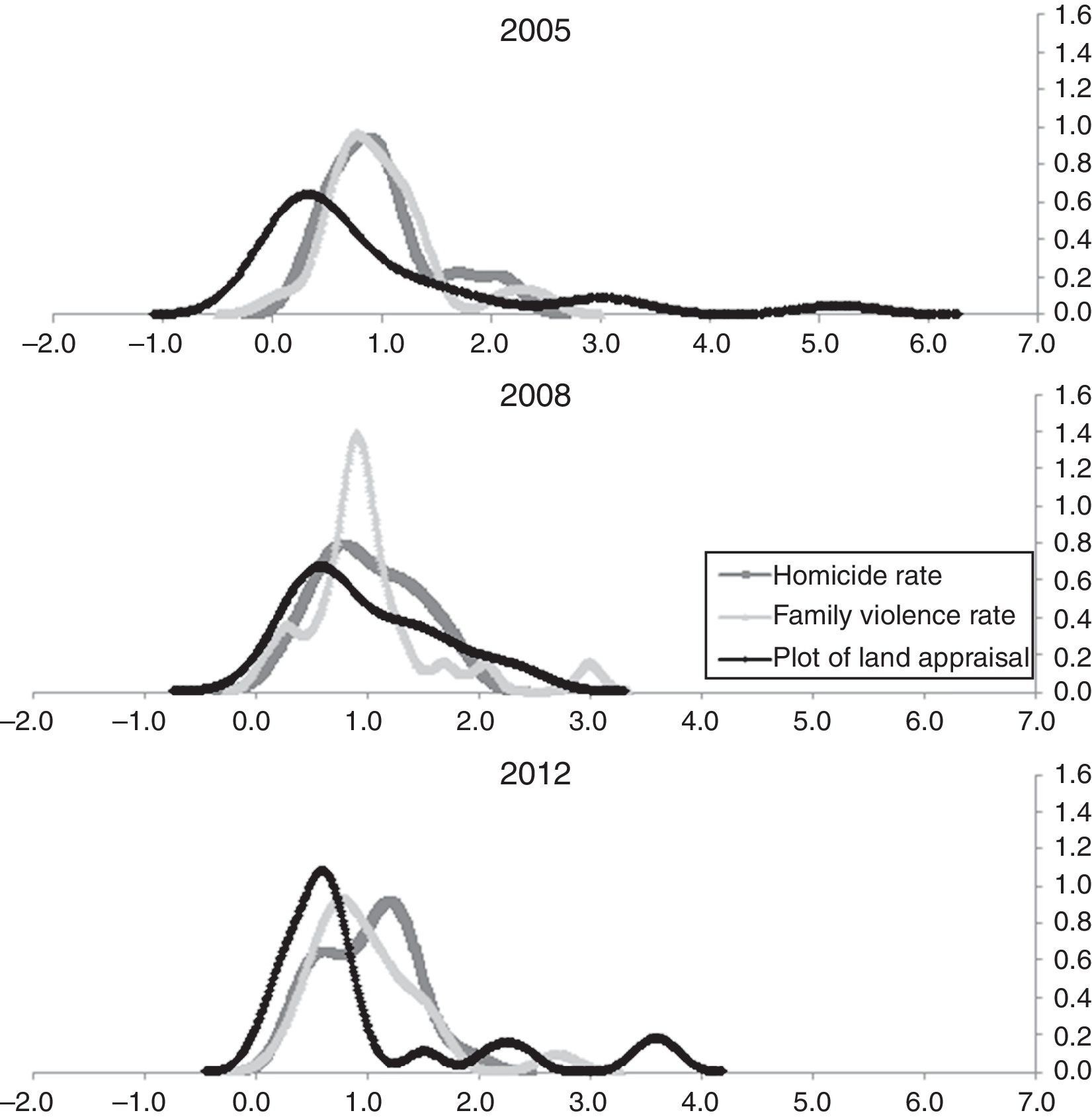
6.2.2Instrument justificationThe use of the instrumental variable is justified by the data, which appear to reveal their positive association with the instrumented variable. The correlation coefficient between the means of the two controls – for the 2005–2015 period – is 0.55; meanwhile, the univariate kernel density estimations show a similar performance in the concentration pattern of the probabilistic mass, especially in 2005 and 2012 (see Fig. 4). Contrary to this, the probabilistic patterns of the land price variable and the instrumental variable seem not to be associated.
 – distribution by communes.")
Gaussian kernels of the principal variables (in all the estimations, we utilize the participation of each observation in the mean of itself) – distribution by communes.
Finally, the use of this variable is also validated by the literature, especially in studies about abuse and intra-home violence. For example, according to Van De Weijer et al. (2015), violent crimes could be a manifestation of an aggressive feature that may also be expressed by aggressive and violent behavior in daily life. It implies that the children of violent parents could have a greater propensity to witness and acquire the violent behavior catalog of their parents than children of non-violent parents.
In other words, crime transmission could be intergenerational and a consequence of social learning mechanisms if the children imitate and adopt the criminal behavior of their parents. Identically, Pollak (2002) presented a theoretical model to predict the effects of being a witness of violence between the parents on the probability that the children will become violent in their own marriages, in the victim or victimizer role.
Complementarily, Van De Weijer et al. (2014) demonstrated that paternal violence during early childhood heightens the risk that individuals will become violent criminals. On the other hand, Loureiro et al. (2009), using data from the state jail in Brazil, estimated by means of the probit model that the variable “was physically abused in excess by your parents” is significant in the explanation of violent crimes such as homicide and rape. Likewise, the logistic regressions run by Herrera and McCloskey (2001), with population data from southwest intermediate cities in the USA, revealed that during the 1990s witnessing marital violence was associated with teenage crime. The same applies to child abuse in relation to violent crimes, especially in young women.
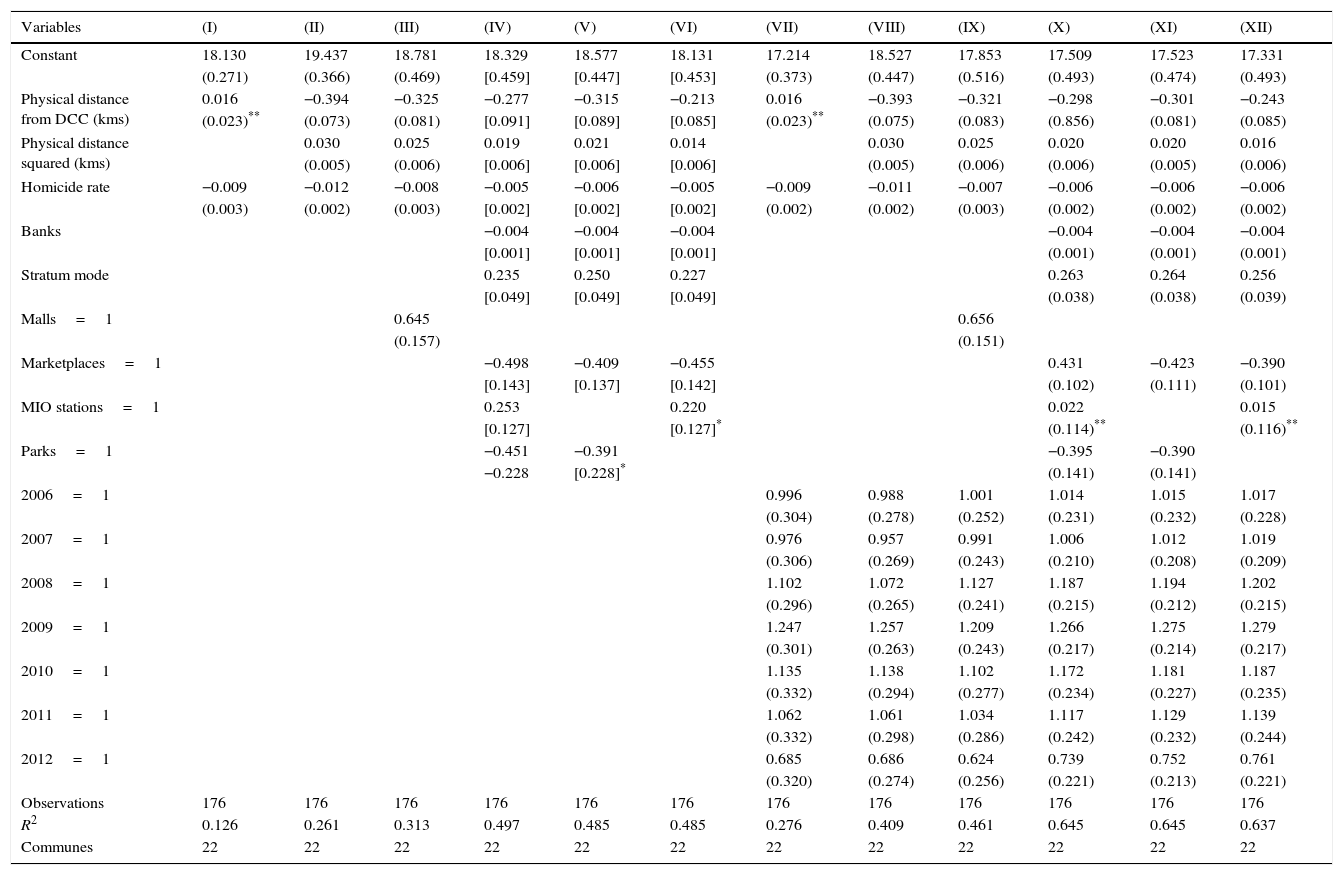
7OLS analysis resultsAccording to Table 2, the presence of malls and public transport stations has a positive effect on the land prices, denoting that proximity to commercial nodes and public mobility equipment that are similar to those localized in the DCC increases land prices. Nevertheless, the presence of banks, marketplaces and large parks has the opposite effect. In the case of banks – measured per area unit – the effect may be due to the values in communes 2 and 20, which were approximated with the values of the nearby communes (1 and 19), and the two commune pairs are very different in their appraisals (see Appendix 1). Consequently, there is a variable that shows the same endowments but in the presence of a notable land price polarization. This also affects the high value in the DCC, the appraisal of which in the observed period is below the mean of all the communes.
Dependent variable: mean appraisal of plot of land per commune (MAPC) in Cali 2005–2012 (in logarithms) – OLS estimation.
| Variables | (I) | (II) | (III) | (IV) | (V) | (VI) | (VII) | (VIII) | (IX) | (X) | (XI) | (XII) |
|---|---|---|---|---|---|---|---|---|---|---|---|---|
| Constant | 18.130 | 19.437 | 18.781 | 18.329 | 18.577 | 18.131 | 17.214 | 18.527 | 17.853 | 17.509 | 17.523 | 17.331 |
| (0.271) | (0.366) | (0.469) | [0.459] | [0.447] | [0.453] | (0.373) | (0.447) | (0.516) | (0.493) | (0.474) | (0.493) | |
| Physical distance from DCC (kms) | 0.016 | −0.394 | −0.325 | −0.277 | −0.315 | −0.213 | 0.016 | −0.393 | −0.321 | −0.298 | −0.301 | −0.243 |
| (0.023)** | (0.073) | (0.081) | [0.091] | [0.089] | [0.085] | (0.023)** | (0.075) | (0.083) | (0.856) | (0.081) | (0.085) | |
| Physical distance squared (kms) | 0.030 | 0.025 | 0.019 | 0.021 | 0.014 | 0.030 | 0.025 | 0.020 | 0.020 | 0.016 | ||
| (0.005) | (0.006) | [0.006] | [0.006] | [0.006] | (0.005) | (0.006) | (0.006) | (0.005) | (0.006) | |||
| Homicide rate | −0.009 | −0.012 | −0.008 | −0.005 | −0.006 | −0.005 | −0.009 | −0.011 | −0.007 | −0.006 | −0.006 | −0.006 |
| (0.003) | (0.002) | (0.003) | [0.002] | [0.002] | [0.002] | (0.002) | (0.002) | (0.003) | (0.002) | (0.002) | (0.002) | |
| Banks | −0.004 | −0.004 | −0.004 | −0.004 | −0.004 | −0.004 | ||||||
| [0.001] | [0.001] | [0.001] | (0.001) | (0.001) | (0.001) | |||||||
| Stratum mode | 0.235 | 0.250 | 0.227 | 0.263 | 0.264 | 0.256 | ||||||
| [0.049] | [0.049] | [0.049] | (0.038) | (0.038) | (0.039) | |||||||
| Malls=1 | 0.645 | 0.656 | ||||||||||
| (0.157) | (0.151) | |||||||||||
| Marketplaces=1 | −0.498 | −0.409 | −0.455 | 0.431 | −0.423 | −0.390 | ||||||
| [0.143] | [0.137] | [0.142] | (0.102) | (0.111) | (0.101) | |||||||
| MIO stations=1 | 0.253 | 0.220 | 0.022 | 0.015 | ||||||||
| [0.127] | [0.127]* | (0.114)** | (0.116)** | |||||||||
| Parks=1 | −0.451 | −0.391 | −0.395 | −0.390 | ||||||||
| −0.228 | [0.228]* | (0.141) | (0.141) | |||||||||
| 2006=1 | 0.996 | 0.988 | 1.001 | 1.014 | 1.015 | 1.017 | ||||||
| (0.304) | (0.278) | (0.252) | (0.231) | (0.232) | (0.228) | |||||||
| 2007=1 | 0.976 | 0.957 | 0.991 | 1.006 | 1.012 | 1.019 | ||||||
| (0.306) | (0.269) | (0.243) | (0.210) | (0.208) | (0.209) | |||||||
| 2008=1 | 1.102 | 1.072 | 1.127 | 1.187 | 1.194 | 1.202 | ||||||
| (0.296) | (0.265) | (0.241) | (0.215) | (0.212) | (0.215) | |||||||
| 2009=1 | 1.247 | 1.257 | 1.209 | 1.266 | 1.275 | 1.279 | ||||||
| (0.301) | (0.263) | (0.243) | (0.217) | (0.214) | (0.217) | |||||||
| 2010=1 | 1.135 | 1.138 | 1.102 | 1.172 | 1.181 | 1.187 | ||||||
| (0.332) | (0.294) | (0.277) | (0.234) | (0.227) | (0.235) | |||||||
| 2011=1 | 1.062 | 1.061 | 1.034 | 1.117 | 1.129 | 1.139 | ||||||
| (0.332) | (0.298) | (0.286) | (0.242) | (0.232) | (0.244) | |||||||
| 2012=1 | 0.685 | 0.686 | 0.624 | 0.739 | 0.752 | 0.761 | ||||||
| (0.320) | (0.274) | (0.256) | (0.221) | (0.213) | (0.221) | |||||||
| Observations | 176 | 176 | 176 | 176 | 176 | 176 | 176 | 176 | 176 | 176 | 176 | 176 |
| R2 | 0.126 | 0.261 | 0.313 | 0.497 | 0.485 | 0.485 | 0.276 | 0.409 | 0.461 | 0.645 | 0.645 | 0.637 |
| Communes | 22 | 22 | 22 | 22 | 22 | 22 | 22 | 22 | 22 | 22 | 22 | 22 |
In the case of parks and marketplaces, the results agree with the explication by Ortiz (2010) as regards the presence of this kind of space, like urban space fractures, which, with an inefficient watch, may be complicit with other kinds of violent crime that generate adverse effects on the real estate prices, which is also consistent with the results exposed by Troy and Grove (2008).
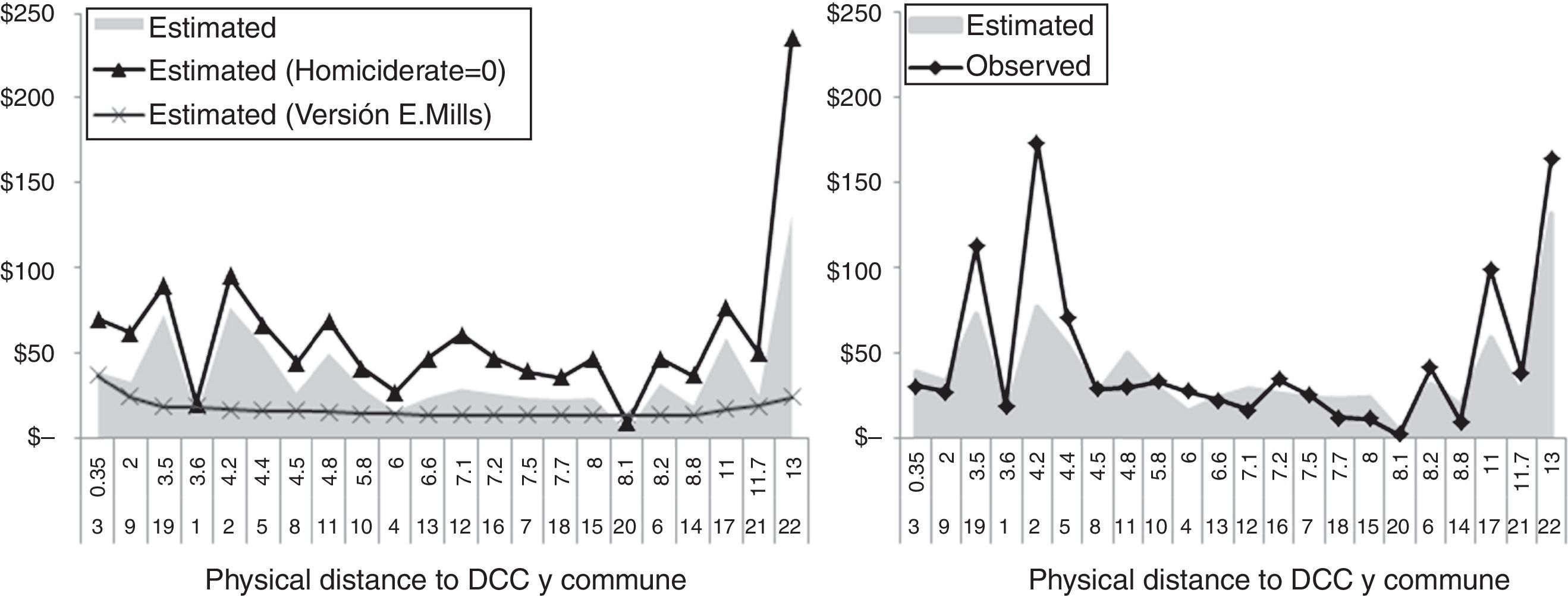
Regarding the physical distance, the signs were as expected; that is, there is a contraction of the mean price per commune with a greater distance from the DCC as well as an increase for distances greater than 7.7km (commune 18) from the same area. This could be calculated from model (XI)10 supposing all the variables except the distance to be null; see Fig. 5a (Mills version). This would show that the city does not have a monocentric structure, although the economic cycle effects expose growth in the appraisals in this zone since 2005. This, additionally, is congruent with the city's expansion to the south zone (communes 17 and 22), which has been accompanied by high appraisals for decades.
 2012 (2008=100) – OLS estimations (COP millions).")
In relation to the variable of interest for this research, the estimation shows that – everything else being constant – it is significant. The estimated parameter evidences that, when the annual homicide rate rises by 1 unit, the MAPC is reduced by a value that oscillates between 0.5% and 1.1%, according to the estimated model. This, besides being consistent with the literature mentioned previously, implies a negative wealth effect that is very important to take as a reference; for example, there were 7 communes with mean homicide rates that exceeded 100 units during the observation period. Even more, if commune 22, which has stratum 6, is excluded from this group, we can see that the others are distributed between stratus 1 and stratus 3, revealing that homicide is a social distance factor that enforces friction on the land price.
Verifying the economic magnitude of this friction in the estimation is important; see again Fig. 5 (left), the series “estimated (homicide rate=0)” – which was created with the estimated parameters in model (XI) calculated with data for the year 2012 – allows us to appreciate the estimated appraisal with that structure supposing that there are no homicides. The gap between such a series and the estimated one, including the real values of the homicide rate, approach a mean value per commune of almost 22 COP million (12.442 USD).11
On the other side, as we anticipated in the methodological section, we ran the Hausman (1978) test (see Appendix 2) and the results evince that (except models II, III, V and VII) we cannot reject the exogeneity hypothesis between the homicide rate and the land prices. In other words, the OLS estimations exposed in this section are consistent.
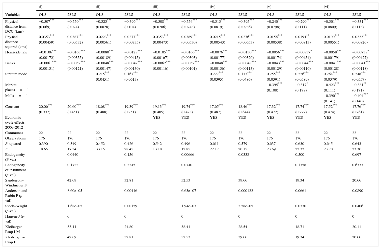
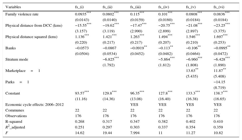
82SLS analysis resultsTo show the research's robustness, we ran regressions following the 2SLS method, employing the family violence rate per commune as an instrumental variable. The results (see Table 3) are even more interesting; however, before analyzing them it is necessary to comment that the reading of the estimations supports statistically the endogeneity hypothesis of the homicide rate in models (i), (iii) and (iv), which is congruent with the Hausman test results in the previous section. It is implied that the OLS estimator may be more efficient in the remaining models. According to the endogeneity test of weakness and under/over-identification of the instrument, there is no evidence of problems in the 2SLS estimations.12 In addition, we present the first-stage estimations (Eq. (6)) in Table 6 in Appendix 3.
Dependent variable: mean appraisal of plot of land per commune (MAPC) in Cali 2005–2012 (in logarithms) Instrumental variable: family violence rate (reported cases per 100,000 people).
| (i) | (ii) | (iii) | (iv) | (v) | (vi) | |||||||
|---|---|---|---|---|---|---|---|---|---|---|---|---|
| Variables | OLS | 2SLS | OLS | 2SLS | OLS | 2SLS | OLS | 2SLS | OLS | 2SLS | OLS | 2SLS |
| Physical distance from DCC (kms) | −0.507*** | −0.550*** | −0.323*** | −0.396*** | −0.508*** | −0.554*** | −0.313*** | −0.395*** | −0.240*** | −0.290*** | −0.301*** | −0.331*** |
| (0.069) | (0.074) | (0.0828) | (0.104) | (0.0706) | (0.0743) | (0.0819) | (0.0936) | (0.0798) | (0.111) | (0.0809) | (0.113) | |
| Physical distance squared (kms) | 0.0353*** | 0.0387*** | 0.0223*** | 0.0277*** | 0.0353*** | 0.0389*** | 0.0215*** | 0.0276*** | 0.0156*** | 0.0194** | 0.0199*** | 0.0222*** |
| (0.00459) | (0.00532) | (0.00561) | (0.00735) | (0.00473) | (0.00530) | (0.00543) | (0.00653) | (0.00538) | (0.00813) | (0.00551) | (0.00826) | |
| Homicide rate | −0.0106*** | −0.0163*** | −0.0080*** | −0.0128*** | −0.0105*** | −0.0166*** | −0.0076*** | −0.0130*** | −0.0056*** | −0.00837* | −0.0058*** | −0.00738* |
| (0.00172) | (0.00355) | (0.00189) | (0.00415) | (0.00167) | (0.00303) | (0.00177) | (0.00326) | (0.00174) | (0.00454) | (0.00179) | (0.00427) | |
| Banks | −0.0061*** | −0.0057*** | −0.0048*** | −0.0047*** | −0.0062*** | −0.0057*** | −0.0048*** | −0.0048*** | −0.0043*** | −0.0044*** | −0.0041*** | −0.0041*** |
| (0.00131) | (0.00121) | (0.00147) | (0.00130) | (0.00116) | (0.00101) | (0.00136) | (0.00113) | (0.00129) | (0.00116) | (0.00128) | (0.00118) | |
| Stratum mode | 0.215*** | 0.167*** | 0.227*** | 0.173*** | 0.255*** | 0.226*** | 0.264*** | 0.248*** | ||||
| (0.0451) | (0.0613) | (0.0395) | (0.0486) | (0.0391) | (0.0589) | (0.0379) | (0.0557) | |||||
| Market places=1 | −0.395*** | −0.317* | −0.423*** | −0.381** | ||||||||
| (0.108) | (0.178) | (0.111) | (0.171) | |||||||||
| Malls=1 | −0.390*** | −0.404*** | ||||||||||
| (0.141) | (0.140) | |||||||||||
| Constant | 20.06*** | 20.60*** | 18.68*** | 19.39*** | 19.13*** | 19.74*** | 17.65*** | 18.46*** | 17.32*** | 17.74*** | 17.52*** | 17.76*** |
| (0.337) | (0.451) | (0.488) | (0.751) | (0.405) | (0.478) | (0.487) | (0.644) | (0.472) | (0.777) | (0.474) | (0.761) | |
| Economic cycle effects: 2006–2012 | YES | YES | YES | YES | YES | YES | YES | YES | ||||
| Communes | 22 | 22 | 22 | 22 | 22 | 22 | 22 | 22 | 22 | 22 | 22 | 22 |
| Observations | 176 | 176 | 176 | 176 | 176 | 176 | 176 | 176 | 176 | 176 | 176 | 176 |
| R-squared | 0.390 | 0.349 | 0.452 | 0.426 | 0.542 | 0.496 | 0.611 | 0.579 | 0.637 | 0.630 | 0.645 | 0.643 |
| F | 18.65 | 17.34 | 33.15 | 28.45 | 13.18 | 12.85 | 22.17 | 20.15 | 23.69 | 22.32 | 23.70 | 23.36 |
| Endogeneity (P-val) | 0.0440 | 0.156 | 0.00666 | 0.0338 | 0.500 | 0.697 | ||||||
| Endogeneity of instrument (p-val) | 0.1722 | 0.3345 | 0.0740 | 0.1758 | 0.6773 | |||||||
| Sanderson–Windmeijer F | 42.69 | 32.81 | 52.53 | 39.66 | 19.34 | 20.66 | ||||||
| Anderson and Rubin F (p-val) | 8.60e−05 | 0.00416 | 6.63e−07 | 0.000122 | 0.0661 | 0.0890 | ||||||
| Stock–Wright (p-val) | 1.68e−05 | 0.00159 | 1.94e−07 | 3.58e−05 | 0.0330 | 0.0406 | ||||||
| Hansen-J (p-val) | 0 | 0 | 0 | 0 | 0 | 0 | ||||||
| Kleibergen–Paap LM | 33.11 | 24.80 | 38.41 | 28.54 | 18.71 | 20.11 | ||||||
| Kleibergen–Paap F | 42.69 | 32.81 | 52.53 | 39.66 | 19.34 | 20.66 | ||||||
The first outcome that arises in contrasting the estimated coefficient of this exercise versus that estimated by OLS is that the results are convergent in terms of significance and expected relationships; thus, the interpretations of each control in the models are the same as those in the previous section.
Secondly, it can be seen that the estimated parameters for the amenities were over-estimated in the OLS model, contrary to the results for the variables associated with physical distance. Seen otherwise, evidence exists that the effect of factors that theoretically reduce the friction on the MAPC is smaller, while the control parameters that would increase the friction are larger. This corroborates the third outcome – the most important one for this paper – which is that the estimated parameter for the homicide rate in all the models was under-estimated, which demonstrates that it is very probable that the effect of this crime modality on the mean value of the land in each commune is even larger. Hence, with the consistent result of the 2SLS estimation, it can be inferred that an increase of one unit in the annual homicide rate could produce a loss in the MAPC of up to 1.66 percentage points.
Finally, a grouped observation of the OLS and 2SLS results allows us to comment, from an economic viewpoint, that homicide's adverse effects exceed a reduction in the real estate value, because in fact they may be more damaging. This applies more to relatively more impoverished communes of lower strata, which are those that historically concentrate the phenomenon in the city. In other words, though the estimated coefficient that measures this negative effect is the same for all the communes, homicide acts as a regressive tax due to it producing proportionally a greater influence on the wealth of the poorest population.
9Conclusion and discussionThis paper – which could be cataloged as a study of the costs of violence – has made a pertinent contribution to the investigative discussion about the adverse effects of homicide on the value of real estate assets in Cali. It is convenient to highlight that this research had not previously been conducted for the city in spite of the complicated scenario of criminality present during recent years.
From the theoretical and technical perspectives, we generated an extended version of the Mills model (1972) that allowed us to introduce homicide as a social distance factor; in addition, we executed OLS estimations – applying the Hausman (1978) test to contrast the endogeneity between homicide and land values – as well as 2SLS estimations using the family violence rate as an instrument, which gave more robustness to the results.
With commune data (2005–2012), the presented model enabled us to provide evidence that the city does not have a monocentric urban structure and that there is no endogeneity between the homicide rate and the land prices. Nevertheless, the most important result is the finding that in both estimation groups – even including amenities – homicide reduced the appraisal values per commune, constituting an important impoverishment mechanism due to the generation of a negative effect on the wealth of real estate proprietors.
Given this, the homicide effect could be seen as a regressive tax with even more perverse consequences because of the spatial concentration in lower-strata areas, the poorest parts of the city, so it may reasonably be assumed to be a factor that systematically extends the social distance within a city and intensifies the problem.
The authors thank the support from Lina Maritza Gómez.
- i.
The physical distances from the DCC were measured in kilometers from each commune central point starting with the shortest terrestrial route based on the Google Maps software.
- ii.
Banks’ quantity was measured in density terms per 1000 hectares (HA). Given that the number of banks in communes 1 and 20 was zero (0), we reasonably suppose that the proxy for this variable is the banks in the nearest communes, that is, 1 and 19.
- iii.
Some appraisal data per commune were outliers or seemed to be badly typed in the Cali en Cifras documents, so they were averaged using the previous and subsequent observations (communes 19 and 21 in 2006 and communes 7 and 21 in 2005).
- iv.
Marketplaces are public spaces to commercialize farm and food products as well as crafts and other home elements.
- v.
It considers as large parks those with areas that exceed 100,000m2. This criterion is due to the existence of an abundance of these spaces in the city, but large parks are few and, hence, could have a differential effect on the land prices.
- vi.
The family violence cases for commune 22 between 2005 and 2007 were approximated with the 2008 value due to this period being included in the observations of commune 17. Naturally, later they were deducted from commune 17 to avoid double counting.
See Table 4.
Selection model statistics and the Hausman endogeneity test in OLS estimations.
| Statistics | (I) | (II) | (III) | (IV) | (V) | (VI) | (VII) | (VIII) | (IX) | (X) | (XI) | (XII) |
|---|---|---|---|---|---|---|---|---|---|---|---|---|
| Bayesian (BIC) | 478.8 | 454.5 | 446.7 | 412.7 | 411.7 | 411.6 | 482.0 | 451.3 | 440.0 | 387.2 | 382.1 | 386.4 |
| Akaike (AIC) | 469.3 | 441.8 | 430.8 | 384.2 | 386.3 | 386.2 | 450.3 | 416.4 | 402.0 | 336.5 | 334.5 | 338.9 |
| Hausman (Prob>Chi2) | 0.986 | 0.002 | 0.001 | 0.177 | 0.023 | 0.151 | 0.808 | 0.029 | 0.063 | 0.389 | 0.195 | 0.381 |
Lower BIC and AIC statistics indicate a better adjustment of the model. Hausman: if Prob >0.05, there are no systematic differences in the coefficients; that is, the variable “homicide rate” is exogenous.
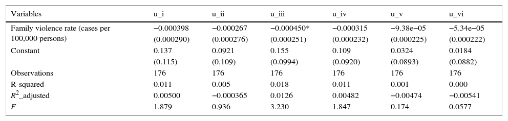
See Tables 5 and 6.
Auxiliary regression estimations. Dependent variables: predicted errors in the OLS estimations of Table 3.
| Variables | u_i | u_ii | u_iii | u_iv | u_v | u_vi |
|---|---|---|---|---|---|---|
| Family violence rate (cases per 100,000 persons) | −0.000398 | −0.000267 | −0.000450* | −0.000315 | −9.38e−05 | −5.34e−05 |
| (0.000290) | (0.000276) | (0.000251) | (0.000232) | (0.000225) | (0.000222) | |
| Constant | 0.137 | 0.0921 | 0.155 | 0.109 | 0.0324 | 0.0184 |
| (0.115) | (0.109) | (0.0994) | (0.0920) | (0.0893) | (0.0882) | |
| Observations | 176 | 176 | 176 | 176 | 176 | 176 |
| R-squared | 0.011 | 0.005 | 0.018 | 0.011 | 0.001 | 0.000 |
| R2_adjusted | 0.00500 | −0.000365 | 0.0126 | 0.00482 | −0.00474 | −0.00541 |
| F | 1.879 | 0.936 | 3.230 | 1.847 | 0.174 | 0.0577 |
Robust standard errors in parenthesis.
*p<0.1.
First-stage estimations in 2SLS models. Dependent variable: homicide rate (reported cases per 100,000 people per Cali commune 2005–2012).
| Variables | fs_(i) | fs_(ii) | fs_(iii) | fs_(iv) | fs_(v) | fs_(vi) |
|---|---|---|---|---|---|---|
| Family violence rate | 0.0935*** | 0.0802*** | 0.115*** | 0.101*** | 0.0808*** | 0.0836*** |
| (0.0143) | (0.0140) | (0.0159) | (0.0160) | (0.0184) | (0.0184) | |
| Physical distance from DCC (kms) | −15.55*** | −19.62*** | −17.47*** | −20.75*** | −21.08*** | −23.25*** |
| (3.157) | (3.119) | (2.990) | (2.899) | (2.897) | (3.375) | |
| Physical distance squared (kms) | 1.136*** | 1.421*** | 1.263*** | 1.494*** | 1.546*** | 1.697*** |
| (0.220) | (0.217) | (0.217) | (0.207) | (0.210) | (0.253) | |
| Banks | −0.0573 | −0.0867 | −0.0919** | −0.113** | −0.106** | −0.0995** |
| (0.0504) | (0.0534) | (0.0452) | (0.0482) | (0.0464) | (0.0472) | |
| Stratum mode | −6.825*** | −5.864*** | −6.960*** | −6.428*** | ||
| (1.792) | (1.812) | (1.808) | (1.890) | |||
| Marketplace=1 | 13.63** | 11.87** | ||||
| (5.435) | (5.408) | |||||
| Parks=1 | −14.15 | |||||
| (8.719) | ||||||
| Constant | 93.57*** | 129.8*** | 96.35*** | 127.8*** | 133.3*** | 138.7*** |
| (11.16) | (14.36) | (13.08) | (16.40) | (16.38) | (16.65) | |
| Economic cycle effects: 2006–2012 | YES | YES | YES | YES | ||
| Communes | 22 | 22 | 22 | 22 | 22 | 22 |
| Observations | 176 | 176 | 176 | 176 | 176 | 176 |
| R-squared | 0.268 | 0.317 | 0.347 | 0.382 | 0.402 | 0.410 |
| R2_adjusted | 0.251 | 0.297 | 0.303 | 0.337 | 0.354 | 0.359 |
| F | 14.62 | 19.44 | 7.994 | 11 | 11.27 | 10.82 |
Robust standard errors in parenthesis.
*p<0.1.
Bogardus (1965) defined it as the degrees of understanding and sympathy between people, between people and social groups, and among social groups.
The group of cities and metropolitan areas defined by the National Administrative Department of Statistics (DANE) for some of its statistical operations. It consists of Bogotá, Medellín, Cali, Barranquilla, Bucaramanga, Manizales, Pasto, Pereira, Cúcuta, Montería, Neiva, Cartagena and Villavicencio.
The standard deviations were in the following order: Cali: 10.6, Medellin: 54.6, Pereira: 22 and Cucuta: 31.7.
Cadastral appraisal: the value of properties for tax purposes and fiscal relations with the State.
This classic model determines the collective configuration about land use and rent, of which the main feature is the manufacturers’ concentration in a central city (Masahisa et al., 1999).
Following the concepts of the original Mills model, β3 can be called the “price – social distance gradient” and in this study the “price – homicide gradient.”
Cali en Cifras is a publication of the Municipal Planning Department of the Mayor's office in Cali, which collects data from different sources and indicators about the city with a one-year lag.
This is equal to saying that the lineal function has an intercept.
In the case of one instrument, its value is equal to the Cragg–Donald Wald test (when the errors are homoskedastic) or the Kleiberger–Paap Wald test (with standard errors that are robust to heteroskedasticity).