


This paper presents empirical evidence on the interrelationship that exists between the evolution of the Emerging Markets Bonds Index (EMBI) and some macroeconomic variables in seven Latin American countries; two of them (Ecuador and Panama), full dollarized. We make use of a Cointegrated Vector framework to analyze the short run effects from 2001 to 2009. The results suggest that EMBI is more stable in dollarized countries and that its evolution influences economic activity in non-dollarized economies; suggesting that investors’ confidence might be higher in dollarized countries where real and financial economic evolution are less vulnerable to external shocks than in non-dollarized ones.
Este documento aporta la evidencia empírica de la interrelación existente entre la evolución del Indicador de Bonos de Mercados Emergentes y ciertas variables macroeconómicas en 7 países latinoamericanos, de entre los cuales 2 de ellos (Ecuador y Panamá), están plenamente dolarizados. Utilizamos el marco del vector cointegrado para analizar los efectos a corto plazo desde 2001 a 2009. Los resultados indican que el Indicador de Bonos de Mercados Emergentes es más estable en los países dolarizados, y que su evolución ejerce una influencia sobre la actividad económica de las economías no dolarizadas, lo cual apunta a que la confianza de los inversores pudiera ser superior en los países dolarizados, donde la evolución económica real y financiera es menos vulnerable a los shocks externos que en los países no dolarizados.
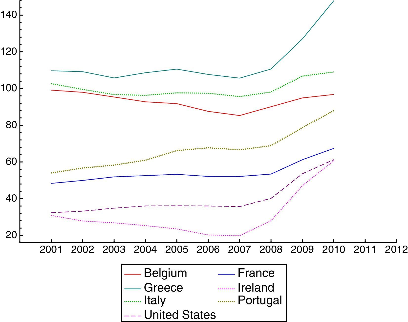
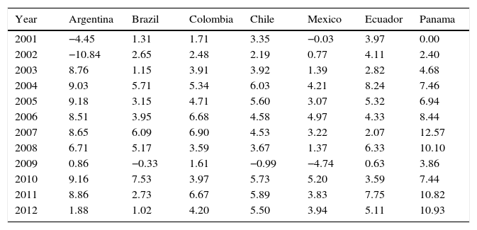
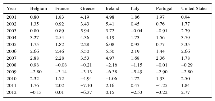
The global financial and economic crisis of 2008–2009 had a much smaller impact on emerging Latin American markets than on their US and European counterparts. While Latin American countries have continued to grow and do not present major macroeconomic imbalances, the advanced economies still do not present solid recovery (Figs. 1 and 2 jointly with Tables 1 and 2, show the evolution of GDP growth and of the government-debt-to-GDP ratio in the two groups of countries). The marginal exposure of banks in emerging markets to US subprime assets and their governments’ expansive monetary and fiscal policies to stimulate aggregate demand might explain these differences (see Aizenman et al., 2013). However, some authors have analyzed whether exchange rate regimes have played a part.1
. (Latin American countries’ evolution.)")
. (Evolution of the US and European countries.)")
Annual GDP rate of growth.
| Year | Argentina | Brazil | Colombia | Chile | Mexico | Ecuador | Panama |
|---|---|---|---|---|---|---|---|
| 2001 | −4.45 | 1.31 | 1.71 | 3.35 | −0.03 | 3.97 | 0.00 |
| 2002 | −10.84 | 2.65 | 2.48 | 2.19 | 0.77 | 4.11 | 2.40 |
| 2003 | 8.76 | 1.15 | 3.91 | 3.92 | 1.39 | 2.82 | 4.68 |
| 2004 | 9.03 | 5.71 | 5.34 | 6.03 | 4.21 | 8.24 | 7.46 |
| 2005 | 9.18 | 3.15 | 4.71 | 5.60 | 3.07 | 5.32 | 6.94 |
| 2006 | 8.51 | 3.95 | 6.68 | 4.58 | 4.97 | 4.33 | 8.44 |
| 2007 | 8.65 | 6.09 | 6.90 | 4.53 | 3.22 | 2.07 | 12.57 |
| 2008 | 6.71 | 5.17 | 3.59 | 3.67 | 1.37 | 6.33 | 10.10 |
| 2009 | 0.86 | −0.33 | 1.61 | −0.99 | −4.74 | 0.63 | 3.86 |
| 2010 | 9.16 | 7.53 | 3.97 | 5.73 | 5.20 | 3.59 | 7.44 |
| 2011 | 8.86 | 2.73 | 6.67 | 5.89 | 3.83 | 7.75 | 10.82 |
| 2012 | 1.88 | 1.02 | 4.20 | 5.50 | 3.94 | 5.11 | 10.93 |
Annual GDP rate of growth.
| Year | Belgium | France | Greece | Ireland | Italy | Portugal | United States |
|---|---|---|---|---|---|---|---|
| 2001 | 0.80 | 1.83 | 4.19 | 4.98 | 1.86 | 1.97 | 0.94 |
| 2002 | 1.35 | 0.92 | 3.43 | 5.41 | 0.45 | 0.76 | 1.77 |
| 2003 | 0.80 | 0.89 | 5.94 | 3.72 | −0.04 | −0.91 | 2.79 |
| 2004 | 3.27 | 2.54 | 4.36 | 4.19 | 1.73 | 1.56 | 3.79 |
| 2005 | 1.75 | 1.82 | 2.28 | 6.08 | 0.93 | 0.77 | 3.35 |
| 2006 | 2.66 | 2.46 | 5.50 | 5.50 | 2.19 | 1.44 | 2.66 |
| 2007 | 2.88 | 2.28 | 3.53 | 4.97 | 1.68 | 2.36 | 1.78 |
| 2008 | 0.98 | −0.08 | −0.21 | −2.16 | −1.15 | −0.01 | −0.29 |
| 2009 | −2.80 | −3.14 | −3.13 | −6.38 | −5.49 | −2.90 | −2.80 |
| 2010 | 2.32 | 1.72 | −4.94 | −1.06 | 1.72 | 1.93 | 2.50 |
| 2011 | 1.76 | 2.02 | −7.10 | 2.16 | 0.47 | −1.25 | 1.84 |
| 2012 | −0.13 | 0.01 | −6.37 | 0.15 | −2.53 | −3.22 | 2.77 |
This paper has two main objectives. The first is to empirically investigate the role of fundamentals in the reduced vulnerability to shocks observed in the bond markets of seven Latin American countries, and how this reduced vulnerability has in turn affected macroeconomic fundamentals. The second is to determine whether there are any differences between countries that can be attributed to their exchange rate regime. Specifically, we aim to compare countries with and without a fully-dollarized economy. To this end, we empirically assess the relationship between key economic factors such as the external debt-to-exports ratio and inflation, and the Emerging Markets Bonds Index (EMBI)2 during the sample period 2001–2009. In the second stage of the study, we aim to establish whether there are relevant differences in the two groups of countries (dollarized and non-dollarized economies).
A review of the empirical literature shows that our first question has usually been approached through an analysis of the main determinants of country risk premium.3 For instance, Edwards (1986) uses data on yields of 167 bonds floated by 13 Least Developed Countries (LDC) between 1976 and 1980 to analyze the factors that determine the country risk premium. He presents evidence that bond spreads depend positively on the countries’ level of indebtedness and negatively on the level of investment they undertake. Nogués and Grandes (2001), focusing on monthly data for Argentina between 1994 and 1998 and estimating its econometric model by OLS, conclude that endogenous factors such as the external debt-to-exports ratio, the fiscal deficit, growth expectations, contagion effects or political noise are the determinants of Argentina's country risk. Gónzalez-Rozada and Levy Yeyati (2008), however, estimating panel error-correction models of emerging spreads on high-yield corporate bonds in developed markets and international rates (US Treasury bills) and using high frequency (monthly, weekly and daily) data from 33 emerging economies, find that global (exogenous) factors explain over 50 per cent of the long run volatility of emerging market spreads.
To sum up, the country risk premium has generally been proxied in the literature by sovereign spreads. Specifically, the spread of JP Morgan's EMBI Global index over US Treasuries bills in Latin America countries is the most important reference for prospective investors in this area.
The research so far on the determinants of country risk can be classified in three groups.4 First, certain authors have found a significant correlation between macroeconomic-political variables and the risk premium (Hoti and McAller, 2004; Baldacci et al., 2008; Aizenman et al., 2013). Authors in the second group have emphasized the effect of exogenous factors (global factors, contagion effects, capital flows or “investor's sentiment”) on risk premium (Eichengreen and Mody, 1998; Kamin and Von Kleist, 1999; Schuknecht et al., 2009, 2010). Finally, authors in the third group relate country risk and the exchange rate regime. They consider that investors want to know two major components of country risk premium: the currency premium, which can be measured as the yield spread between non-dollar-denominated and US dollar-denominated sovereign debt of the same borrowing country, and the credit premium, measured as the yield spread between the dollar-denominated sovereign debt of the emerging country and US Treasury bills. There is a certain consensus inside the third group of authors that dollarization and hard pegs would substantially reduce the country risk of emerging countries (Domowitz et al., 1998; Rubinstein, 1999; Schmukler, 2002).
The aim of this paper is to contribute to this branch of the literature by examining the impact of macroeconomic fundamentals on risk premium and vice versa, since movements in government bond yields may have significant macroeconomic consequences, (see Caceres et al., 2010).
The literature on the determinants of EMBI in specific Latin American countries is still scarce. Fracasso (2007), a good reference for Brazil (he shows that foreign investors’ appetite for risk impacts substantially on EMBI spreads)5; Nogués and Grandes (2001) for Argentina, who highlight that devaluation risk elimination may not have a statistically significant impact on country risk (other macroeconomic variables such as the external debt-to-exports ratio and growth expectations present a higher impact); Vargas et al. (2012), for Colombia, who present evidence that improvement of fiscal variables reduces the sovereign risk premium; López Herrera et al. (2013) for Mexico, who find long-run relationships between domestic macroeconomic variables and the Mexican EMBI; Lindao Jurado and Erazo Blum (2009) for Ecuador who conclude that debt and the inflation are the most important factors for explaining its country risk; Délano and Selaive (2005), who examine Chilean's EMBI behaviour and conclude that approximately 25% of the variability of the sovereign spread is due to global factors, and finally the IMF (2010) which emphasizes that achieving investment grade lowers Panamanian debt spreads by over 140 basis points.
The rest of the paper is organized as follows. Section 2 discusses the theoretical framework while Section 3 outlines the data and the econometric model used in the empirical analysis. Section 4 reports the main empirical results, comparing dollarized and non-dollarized countries. Finally, Section 5 presents the main conclusions.
2Country risk and EMBI determinants2.1The equilibrium condition for a risk-neutral lenderFollowing Edwards (1986), in an emerging or developing country that cannot affect the world interest rate, the cost of external funds is formed by two concepts: (1) the risk-free world interest rate (i*) and (2) a country risk premium (s) related to the probability of default perceived by the lender (p). In the case of a one-period loan, where in case of default the lender loses both the principal and the interest, the equilibrium condition for a risk-neutral lender is:

From here, the country risk premium is:
where k=1+i*.
Since the probability of default depends positively on the debt-to-GDP ratio, as the seminal article by Eaton and Gersowitz (1981) demonstrated, the country then faces an upwards-sloping supply curve for foreign funds. As the probability of default approaches one, the country risk premium approaches infinity and a credit ceiling will be reached. The country in question will have difficulties gaining access to the world's credit market. If the variables that comprise the probability of default perceived by lenders were known, the countries might be able to improve them in order to reduce it to zero.
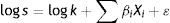
According to Edwards (1986), p has the following logistic function:
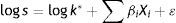
where Xi are the determinants of the sovereign risk premium and βi are the corresponding coefficients. Combining (2) and (3), taking logarithms and adding a random disturbance ¿, the equation to be estimated is: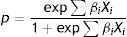
The signs of this equation change slightly if the model is described in terms of returns. Transforming Eq. (1), we obtain:
where r* is the risk-free world return and s represents, this time, the reduction in terms of return on the bond investment, and k*=1+r*. Our Eq. (4) then only changes the signs:
Moving terms, we obtain the emerging country return depending on the same determinants of country risk:
2.2Determinants of each country return index
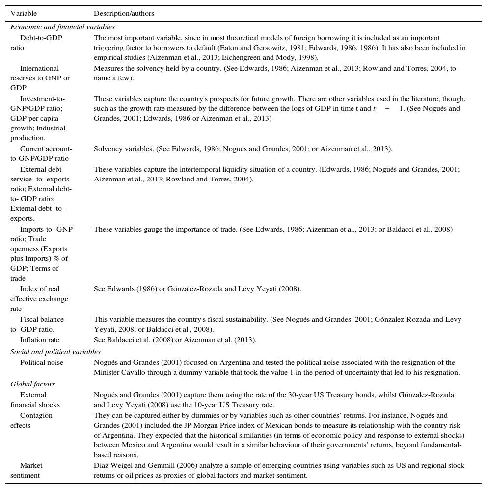
Both theoretical and empirical studies have highlighted a large number of variables that may affect the evolution of government debt returns in emerging countries.6 We can split these variables into three groups: economic-financial, socio-political, and global factors.
Table 3 details some of the variables used in the empirical literature by a wide range of authors to explain the determinants of government debt returns in emerging countries, whilst Table 4 describes the variables used in our model.
Variables used in the literature on sovereign returns’ analysis in emerging countries.
| Variable | Description/authors |
|---|---|
| Economic and financial variables | |
| Debt-to-GDP ratio | The most important variable, since in most theoretical models of foreign borrowing it is included as an important triggering factor to borrowers to default (Eaton and Gersowitz, 1981; Edwards, 1986, 1986). It has also been included in empirical studies (Aizenman et al., 2013; Eichengreen and Mody, 1998). |
| International reserves to GNP or GDP | Measures the solvency held by a country. (See Edwards, 1986; Aizenman et al., 2013; Rowland and Torres, 2004, to name a few). |
| Investment-to-GNP/GDP ratio; GDP per capita growth; Industrial production. | These variables capture the country's prospects for future growth. There are other variables used in the literature, though, such as the growth rate measured by the difference between the logs of GDP in time t and t−1. (See Nogués and Grandes, 2001; Edwards, 1986 or Aizenman et al., 2013) |
| Current account-to-GNP/GDP ratio | Solvency variables. (See Edwards, 1986; Nogués and Grandes, 2001; or Aizenman et al., 2013). |
| External debt service- to- exports ratio; External debt- to- GDP ratio; External debt- to- exports. | These variables capture the intertemporal liquidity situation of a country. (Edwards, 1986; Nogués and Grandes, 2001; Aizenman et al., 2013; Rowland and Torres, 2004). |
| Imports-to- GNP ratio; Trade openness (Exports plus Imports) % of GDP; Terms of trade | These variables gauge the importance of trade. (See Edwards, 1986; Aizenman et al., 2013; or Baldacci et al., 2008) |
| Index of real effective exchange rate | See Edwards (1986) or Gónzalez-Rozada and Levy Yeyati (2008). |
| Fiscal balance- to- GDP ratio. | This variable measures the country's fiscal sustainability. (See Nogués and Grandes, 2001; Gónzalez-Rozada and Levy Yeyati, 2008; or Baldacci et al., 2008). |
| Inflation rate | See Baldacci et al. (2008) or Aizenman et al. (2013). |
| Social and political variables | |
| Political noise | Nogués and Grandes (2001) focused on Argentina and tested the political noise associated with the resignation of the Minister Cavallo through a dummy variable that took the value 1 in the period of uncertainty that led to his resignation. |
| Global factors | |
| External financial shocks | Nogués and Grandes (2001) capture them using the rate of the 30-year US Treasury bonds, whilst Gónzalez-Rozada and Levy Yeyati (2008) use the 10-year US Treasury rate. |
| Contagion effects | They can be captured either by dummies or by variables such as other countries’ returns. For instance, Nogués and Grandes (2001) included the JP Morgan Price index of Mexican bonds to measure its relationship with the country risk of Argentina. They expected that the historical similarities (in terms of economic policy and response to external shocks) between Mexico and Argentina would result in a similar behaviour of their governments’ returns, beyond fundamental-based reasons. |
| Market sentiment | Diaz Weigel and Gemmill (2006) analyze a sample of emerging countries using variables such as US and regional stock returns or oil prices as proxies of global factors and market sentiment. |
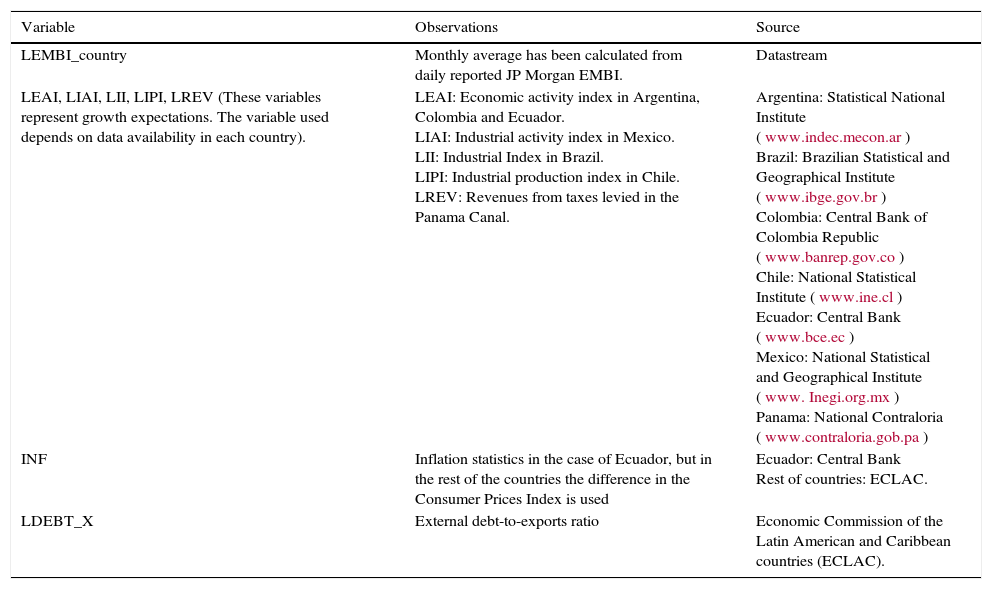
Variables used in our comparative study.
| Variable | Observations | Source |
|---|---|---|
| LEMBI_country | Monthly average has been calculated from daily reported JP Morgan EMBI. | Datastream |
| LEAI, LIAI, LII, LIPI, LREV (These variables represent growth expectations. The variable used depends on data availability in each country). | LEAI: Economic activity index in Argentina, Colombia and Ecuador. LIAI: Industrial activity index in Mexico. LII: Industrial Index in Brazil. LIPI: Industrial production index in Chile. LREV: Revenues from taxes levied in the Panama Canal. | Argentina: Statistical National Institute (www.indec.mecon.ar) Brazil: Brazilian Statistical and Geographical Institute (www.ibge.gov.br) Colombia: Central Bank of Colombia Republic (www.banrep.gov.co) Chile: National Statistical Institute (www.ine.cl) Ecuador: Central Bank (www.bce.ec) Mexico: National Statistical and Geographical Institute (www. Inegi.org.mx) Panama: National Contraloria (www.contraloria.gob.pa) |
| INF | Inflation statistics in the case of Ecuador, but in the rest of the countries the difference in the Consumer Prices Index is used | Ecuador: Central Bank Rest of countries: ECLAC. |
| LDEBT_X | External debt-to-exports ratio | Economic Commission of the Latin American and Caribbean countries (ECLAC). |
Table 4 provides the description of the variables along with the data sources. We included four endogenous variables in our econometric model. The EMBI (with its monthly average calculated from daily data, in order to eliminate its heteroscedasticity and because the rest of variables are available at this frequency), along with variables that are only reported monthly, such as the Economic Activity Index (eai). This variable was used to measure the growth perspective in the case of Argentina, Colombia and Ecuador, while the growth perspective was proxied by the Industrial Activity Index (iai) in Mexico, the Industrial Index (ii) in Brazil, the Industrial Production Index (ipi) in Chile and, finally, the revenues from taxes to cross the Canal in the case of Panama.7 In Panama we used this variable because all the other sectors of its economy depend on Canal activities, as do other markets such as the labour market. The other monthly variables are the inflation rate (inf), which was has been calculated from the Consumer Price Index in all the countries, except in Ecuador where it was directly recorded, and the external debt-to-exports ratio (debt_x), which captures the current account solvency of emerging countries.
The impact of global risk factors will be captured through the inclusion of dummies.
3.2Econometric approach: identification of the short run structure in the Cointegrated VAR (CVAR)Consider the Cointegrated VAR model in the so-called reduced form representation:

Pre-multiplying (8) with a non-singular p×p matrix A0, we obtain the so-called structural form representation:
where A1=A0Г1, a=A0α, vt=A0¿t
The short run equations consist of p equations between p current variables, Δxt, p(k−1) lagged variables (Δxt−i, i=1, …, k−1), and r lagged equilibrium errors, (βc)′xt−1. Identification of the r long run relationships requires at least r−1 restrictions on each relationship, while identification of the simultaneous short run structure of the p equations requires at least p−1 restrictions on each equation.
Keeping the properly identified cointegrating relationships fixed at their estimated values, i.e. by treating (βc)′xt−1 as predetermined stationary regressors, as in the case of Δxt−i, it is easier to identify the simultaneous short run structure. We identify the long run relationships first, and then the short run adjustment parameters.
The unrestricted short run reduced form model is identified exactly by the p−1 zero restrictions on each row of A0=I. Further zero restrictions on Г1, α and Φ are over-identifying. Thus, the process of identification consists firstly in individually testing whether all lagged variables, the long run structure, and dummy variables are statistically significant in the system. The next step is to remove the non-significant variables from the system, so that the generally identified model only contains significant coefficients. The significant coefficients will identify the short run adjustment parameters and the long run relationships that affect the dependent variables of our simultaneous equations system which is estimated by maximum likelihood.8
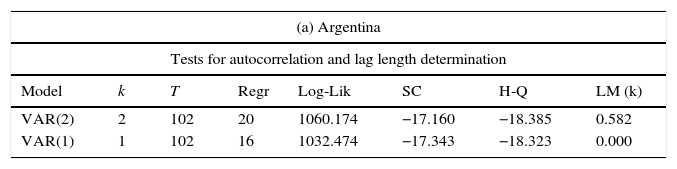
4Empirical results4.1Econometric stepsFirst, we estimated an unrestricted VAR for each country with the following structure: Xt=[EMBI, eai, inf, debt_x]. Previously, all the variables were transformed into logarithms except inflation; recall from Section 3.1 that the variable capturing the growth expectations (eai) changes depending on the country in question. Second, we carried out the residual analysis shown properly in Table 5
Residual analysis.
| (a) Argentina | |||||||
|---|---|---|---|---|---|---|---|
| Tests for autocorrelation and lag length determination | |||||||
| Model | k | T | Regr | Log-Lik | SC | H-Q | LM (k) |
| VAR(2) | 2 | 102 | 20 | 1060.174 | −17.160 | −18.385 | 0.582 |
| VAR(1) | 1 | 102 | 16 | 1032.474 | −17.343 | −18.323 | 0.000 |
| Univariate statistics | |||
|---|---|---|---|
| ARCH(2) | Normality | R-squared | |
| DLEMBI_M_ARG | 3.732 [0.155] | 5.806 [0.055] | 0.697 |
| DLEAI | 0.252 [0.881] | 0.204 [0.903] | 0.945 |
| DINF | 12.131 [0.002] | 4.875 [0.087] | 0.852 |
| DLDEBT_X | 1.473 [0.479] | 17.219 [0.000] | 0.416 |
| (b) Brazil | |||||||
|---|---|---|---|---|---|---|---|
| Tests for autocorrelation and lag length determination | |||||||
| Model | k | T | Regr | Log-Lik | SC | H-Q | LM (k) |
| VAR(3) | 3 | 102 | 13 | 1052.667 | −18.283 | −19.079 | 0.212 |
| VAR(2) | 2 | 102 | 9 | 1031.318 | −18.590 | −19.141 | 0.031 |
| VAR(1) | 1 | 102 | 5 | 1018.918 | −19.072 | −19.378 | 0.151 |
| Univariate statistics | |||
|---|---|---|---|
| ARCH(3) | Normality | R-squared | |
| DLEMBI_M_BRA | 6.537 [0.088] | 7.799 [0.020] | 0.353 |
| DLII | 0.337 [0.953] | 0.048 [0.976] | 0.417 |
| DINF | 1.399 [0.706] | 2.892 [0.236] | 0.516 |
| DLDEBT_X | 5.180 [0.159] | 1.851 [0.396] | 0.336 |
| (c) Colombia | |||||||
|---|---|---|---|---|---|---|---|
| Tests for autocorrelation and lag length determination | |||||||
| Model | k | T | Regr | Log-Lik | SC | H-Q | LM (k) |
| VAR(2) | 2 | 102 | 20 | 946.132 | −14.924 | −16.149 | 0.722 |
| VAR(1) | 1 | 102 | 16 | 909.039 | −14.922 | −15.902 | 0.000 |
| Univariate statistics | |||
|---|---|---|---|
| ARCH(2) | Normality | R-squared | |
| DLEMBI_CO | 2.497 [0.287] | 5.191 [0.075] | 0.501 |
| DLDEBT_X | 1.316 [0.518] | 2.178 [0.337] | 0.553 |
| DLIMACO | 1.075 [0.584] | 9.972 [0.007] | 0.887 |
| DINF | 0.783 [0.676] | 1.328 [0.515] | 0.661 |
| (d) Chile | |||||||
|---|---|---|---|---|---|---|---|
| Tests for autocorrelation and lag length determination | |||||||
| Model | k | T | Regr | Log-Lik | SC | H-Q | LM (k) |
| VAR(3) | 3 | 102 | 24 | 1133.568 | −17.874 | −19.344 | 0.138 |
| VAR(2) | 2 | 102 | 20 | 1107.698 | −18.092 | −19.317 | 0.004 |
| VAR(1) | 1 | 102 | 16 | 1082.957 | −18.332 | −19.313 | 0.001 |
| Univariate statistics | |||
|---|---|---|---|
| ARCH(3) | Normality | R-squared | |
| DLEMBI_CH | 6.776 [0.079] | 1.367 [0.505] | 0.632 |
| DLIPI | 1.186 [0.756] | 0.389 [0.823] | 0.858 |
| DINF | 0.208 [0.976] | 2.704 [0.259] | 0.609 |
| DLDEBT_X | 0.848 [0.838] | 0.252 [0.882] | 0.608 |
| (e) Mexico | |||||||
|---|---|---|---|---|---|---|---|
| Tests for autocorrelation and lag length determination | |||||||
| Model | k | T | Regr | Log-Lik | SC | H-Q | LM (k) |
| VAR(4) | 4 | 102 | 17 | 773.042 | −12.074 | −13.116 | 0.189 |
| VAR(3) | 3 | 102 | 13 | 748.491 | −12.318 | −13.115 | 0.002 |
| VAR(2) | 2 | 102 | 9 | 714.167 | −12.371 | −12.922 | 0.000 |
| VAR(1) | 1 | 102 | 5 | 693.836 | −12.698 | −13.004 | 0.003 |
| Univariate statistics | |||
|---|---|---|---|
| ARCH(4) | Normality | R-squared | |
| DLEMBI_MX | 8.903 [0.064] | 3.879 [0.144] | 0.654 |
| DIAI | 16.944 [0.002] | 1.125 [0.570] | 0.547 |
| DINF | 11.197 [0.024] | 2.921 [0.232] | 0.558 |
| DLDEBT_X | 7.688 [0.104] | 3.403 [0.182] | 0.409 |
| (f) Ecuador | |||||||
|---|---|---|---|---|---|---|---|
| Tests for autocorrelation and lag length determination | |||||||
| Model | k | T | Regr | Log-Lik | SC | H-Q | LM (k) |
| VAR(2) | 2 | 139 | 20 | 1978.853 | −25.633 | −26.635 | 0.081 |
| VAR(1) | 1 | 139 | 16 | 1931.693 | −25.522 | −26.324 | 0.000 |
| Univariate statistics | |||
|---|---|---|---|
| ARCH(2) | Normality | R-squared | |
| DLEMBI_M_EC | 9.820 [0.007] | 12.068 [0.002] | 0.741 |
| DLEAI | 1.248 [0.536] | 0.021 [0.990] | 0.663 |
| DINF | 2.059 [0.357] | 0.065 [0.968] | 0.775 |
| DLDEBT_X | 4.122 [0.127] | 2.100 [0.350] | 0.469 |
| (g) Panama | |||||||
|---|---|---|---|---|---|---|---|
| Tests for autocorrelation and lag length determination | |||||||
| Model | k | T | Regr | Log-Lik | SC | H-Q | LM (k) |
| VAR(2) | 2 | 102 | 20 | 1039.011 | −16.745 | −17.970 | 0.589 |
| VAR(1) | 1 | 102 | 16 | 1016.394 | −17.027 | −18.007 | 0.029 |
| Univariate statistics | |||
|---|---|---|---|
| ARCH(2) | Normality | R-squared | |
| DLEMBI_M_PANA | 1.942 [0.379] | 3.805 [0.149] | 0.614 |
| DLEREV_C | 0.118 [0.943] | 1.647 [0.439] | 0.745 |
| DINF | 3.593 [0.166] | 0.162 [0.922] | 0.634 |
| DLDEBT_X | 0.335 [0.846] | 2.609 [0.271] | 0.617 |
Here we detail the dummies included for each country:
Argentina: The dummy dum0111p (2001:11) takes into account the significant fall in the Global EMBI due to the currency crisis sparked by Argentina's abandoning of the currency board, following public debt default.9 Dum0202p and dum0204p variables capture the consequences of devaluation that generated inflation pressures (ECLAC, 2002). The dum0504p was included to normalize debt_x residuals since at that date external debt experienced a sharp decrease when Argentina launched a debt exchange in 2005.10 Brazil: dum0211p is included to normalize the debt_x residuals. After the 1999 devaluation on the public debt denominated in US dollars, Brazil's debt increased substantially, reaching 50% of total public debt at the end of 2002.11 Colombia: The objective of dum0405p is to normalize the EMBI residuals; three dummies dum0901p, dum0904p and dum0907p represent the impact of the 2008–2009 global crisis on Colombia's economic activity (ECLAC, 2009). Chile: dum0405p which normalizes the EMBI residuals and the dum0901p which normalizes the economic activity variable (ipi) are incorporated in the analysis. Mexico: dum0405p is also included in order to eliminate the outliers of the EMBI's residuals. Ecuador: Five permanent dummies need to be included. Whilst dum0906p is related to Ecuador default in 2009,12 dum0811p is introduced to jointly explain the debt_x and the EMBI evolution. The rest of dummies are dum0109p and dum0301p which are needed to normalize inflation residuals.13 Panama: The dum0401p normalizes residuals of inflation. Prices decreased in the first quarter of 2004, but the trend reverted afterward due to the rise in oil prices and other import products (ECLAC, 2004).
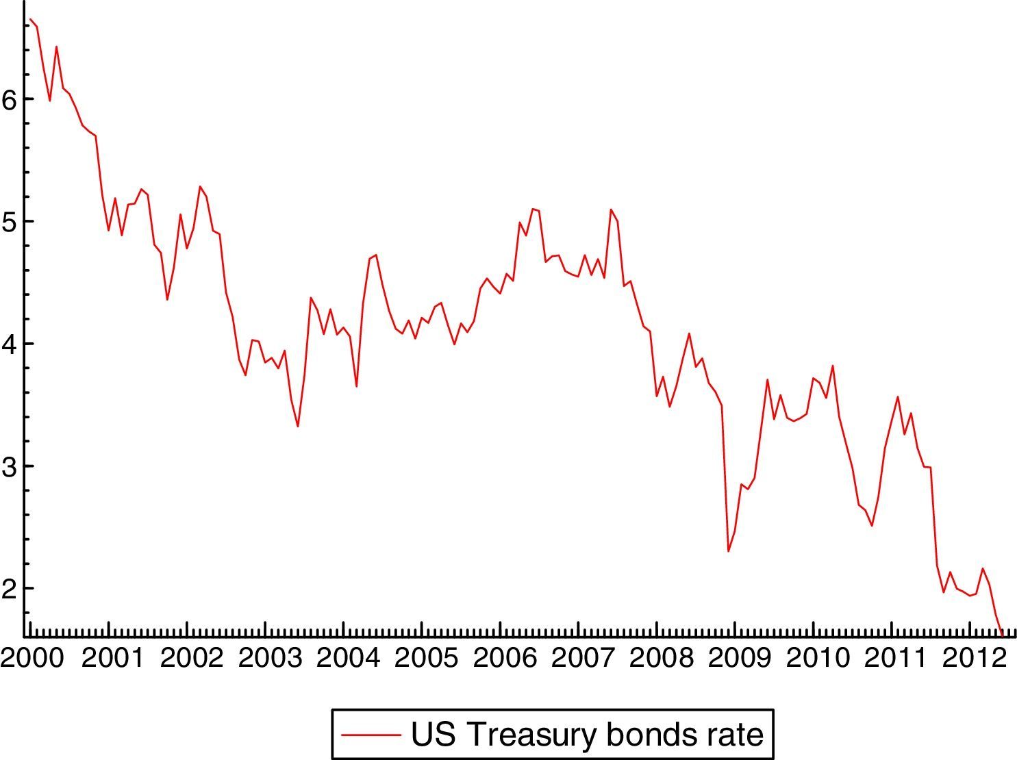
The dum0810p (along with dum0811p only for Ecuador) is common to all the endogenous variables since it is related to the start of the world financial crisis (the US financial institution Lehman Brothers collapsed in September 2008 and affected the EMBI evolution of all emerging countries included in this study). Dummies such as dum0405p and dum0901p might explain contagion effects between Chile, Colombia and Mexico.14 Dum0405p captures the incidence of global factors such as a fall in international interest rates, which we can proxy using the US Treasury 10-year yield15 (Fig. 3 shows that Treasury bonds yields went down in 2004:05).
.")
Following Eichengreen and Mody (1998), we assume that the relationship between the US Treasury bond rates and emerging bond prices is explained in terms of demand.16 On the demand side, when Treasury bonds rates go up (their prices go down), there will be a tendency among investors to substitute emerging bonds by US Treasury bonds, and so the EMBI price falls. Finally, dummy dum0901p represents the vulnerability of Chile and Colombia with respect to the other countries included in the sample during the global economic crisis of 2008–2009.
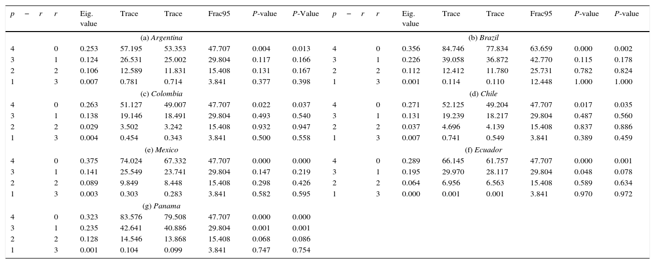
Third, we determined the rank of cointegration; Table 6 shows the results of Johansen's (1996) test, which concludes that all the countries reflect the presence of just one cointegrated vector; so the rank of their long run matrix is equal to 1 (with the exception of Panama, which matrix's rank is 2).
Johansen tests.
| p−r | r | Eig. value | Trace | Trace | Frac95 | P-value | P-Value | p−r | r | Eig. value | Trace | Trace | Frac95 | P-value | P-value |
|---|---|---|---|---|---|---|---|---|---|---|---|---|---|---|---|
| (a) Argentina | (b) Brazil | ||||||||||||||
| 4 | 0 | 0.253 | 57.195 | 53.353 | 47.707 | 0.004 | 0.013 | 4 | 0 | 0.356 | 84.746 | 77.834 | 63.659 | 0.000 | 0.002 |
| 3 | 1 | 0.124 | 26.531 | 25.002 | 29.804 | 0.117 | 0.166 | 3 | 1 | 0.226 | 39.058 | 36.872 | 42.770 | 0.115 | 0.178 |
| 2 | 2 | 0.106 | 12.589 | 11.831 | 15.408 | 0.131 | 0.167 | 2 | 2 | 0.112 | 12.412 | 11.780 | 25.731 | 0.782 | 0.824 |
| 1 | 3 | 0.007 | 0.781 | 0.714 | 3.841 | 0.377 | 0.398 | 1 | 3 | 0.001 | 0.114 | 0.110 | 12.448 | 1.000 | 1.000 |
| (c) Colombia | (d) Chile | ||||||||||||||
| 4 | 0 | 0.263 | 51.127 | 49.007 | 47.707 | 0.022 | 0.037 | 4 | 0 | 0.271 | 52.125 | 49.204 | 47.707 | 0.017 | 0.035 |
| 3 | 1 | 0.138 | 19.146 | 18.491 | 29.804 | 0.493 | 0.540 | 3 | 1 | 0.131 | 19.239 | 18.217 | 29.804 | 0.487 | 0.560 |
| 2 | 2 | 0.029 | 3.502 | 3.242 | 15.408 | 0.932 | 0.947 | 2 | 2 | 0.037 | 4.696 | 4.139 | 15.408 | 0.837 | 0.886 |
| 1 | 3 | 0.004 | 0.454 | 0.343 | 3.841 | 0.500 | 0.558 | 1 | 3 | 0.007 | 0.741 | 0.549 | 3.841 | 0.389 | 0.459 |
| (e) Mexico | (f) Ecuador | ||||||||||||||
| 4 | 0 | 0.375 | 74.024 | 67.332 | 47.707 | 0.000 | 0.000 | 4 | 0 | 0.289 | 66.145 | 61.757 | 47.707 | 0.000 | 0.001 |
| 3 | 1 | 0.141 | 25.549 | 23.741 | 29.804 | 0.147 | 0.219 | 3 | 1 | 0.195 | 29.970 | 28.117 | 29.804 | 0.048 | 0.078 |
| 2 | 2 | 0.089 | 9.849 | 8.448 | 15.408 | 0.298 | 0.426 | 2 | 2 | 0.064 | 6.956 | 6.563 | 15.408 | 0.589 | 0.634 |
| 1 | 3 | 0.003 | 0.303 | 0.283 | 3.841 | 0.582 | 0.595 | 1 | 3 | 0.000 | 0.001 | 0.001 | 3.841 | 0.970 | 0.972 |
| (g) Panama | |||||||||||||||
| 4 | 0 | 0.323 | 83.576 | 79.508 | 47.707 | 0.000 | 0.000 | ||||||||
| 3 | 1 | 0.235 | 42.641 | 40.886 | 29.804 | 0.001 | 0.001 | ||||||||
| 2 | 2 | 0.128 | 14.546 | 13.868 | 15.408 | 0.068 | 0.086 | ||||||||
| 1 | 3 | 0.001 | 0.104 | 0.099 | 3.841 | 0.747 | 0.754 | ||||||||
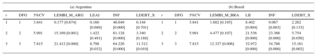
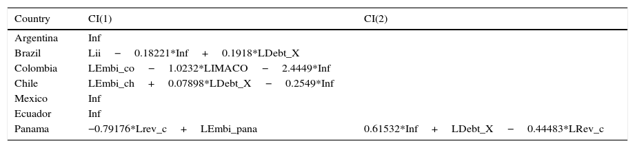
Fourth, we test and impose over-identifying restrictions on the long run structure (beta vectors) in order to have only significant coefficients. Table 7 shows the tests of exclusion for the seven countries, and Table 8 the final cointegration relationships for each of the countries. These long run relationships will be added as another predetermined variable into the simultaneous equation system and, along with dummies and lagged differenced variables, we will test whether their coefficients are significant or not.17
Exclusion tests.
| (a) Argentina | (b) Brazil | ||||||||||||
|---|---|---|---|---|---|---|---|---|---|---|---|---|---|
| r | DFG | 5%CV | LEMBI_M_ARG | LEAI | INF | LDEBT_X | r | DFG | 5%CV | LEMBI_M_BRA | LII | INF | LDEBT_X |
| 1 | 1 | 3.841 | 0.177 [0.674] | 0.160 [0.689] | 46.649 [0.000] | 0.148 [0.701] | 1 | 1 | 3.841 | 1.682 [0.195] | 8.402 [0.004] | 9.067 [0.003] | 2.262 [0.133] |
| 2 | 2 | 5.991 | 15.169 [0.001] | 1.422 [0.491] | 61.128 [0.000] | 3.340 [0.188] | 2 | 2 | 5.991 | 4.477 [0.107] | 21.536 [0.000] | 23.366 [0.000] | 5.754 [0.056] |
| 3 | 3 | 7.815 | 21.412 [0.000] | 8.798 [0.032] | 64.226 [0.000] | 11.312 [0.010] | 3 | 3 | 7.815 | 12.327 [0.006] | 32.972 [0.000] | 34.786 [0.000] | 15.161 [0.002] |
| (c) Colombia | (d) Chile | ||||||||||||
|---|---|---|---|---|---|---|---|---|---|---|---|---|---|
| r | DFG | 5%CV | LEMBI_CO | LIMACO | INF | LDEBT_X | r | DFG | 5%CV | LEMBI_CH | LIPI | INF | LDEBT_X |
| 1 | 1 | 3.841 | 6.244 [0.012] | 11.050 [0.001] | 2.505 [0.113] | 3.386 [0.066] | 1 | 1 | 3.841 | 3.280 [0.070] | 10.785 [0.001] | 12.279 [0.000] | 4.749 [0.029] |
| 2 | 2 | 5.991 | 6.793 [0.033] | 18.160 [0.000] | 17.016 [0.000] | 3.791 [0.150] | 2 | 2 | 5.991 | 5.856 [0.053] | 16.712 [0.000] | 18.250 [0.000] | 8.666 [0.013] |
| 3 | 3 | 7.815 | 18.919 [0.000] | 30.095 [0.000] | 29.917 [0.000] | 15.027 [0.002] | 3 | 3 | 7.815 | 8.233 [0.041] | 19.840 [0.000] | 21.572 [0.000] | 12.050 [0.007] |
| (e) Mexico | (f) Ecuador | ||||||||||||
|---|---|---|---|---|---|---|---|---|---|---|---|---|---|
| r | DFG | 5%CV | LEMBI_MX | IAI | INF | LDEBT_X | r | DFG | 5%CV | LEMBI_M_EC | LEAI | INF | LDEBT_X |
| 1 | 1 | 3.841 | 0.002 [0.961] | 0.015 [0.904] | 32.296 [0.000] | 0.726 [0.394] | 1 | 1 | 3.841 | 1.391 [0.238] | 0.019 [0.891] | 32.046 [0.000] | 0.176 [0.675] |
| 2 | 2 | 5.991 | 1.885 [0.390] | 0.048 [0.976] | 38.251 [0.000] | 4.239 [0.120] | 2 | 2 | 5.991 | 1.429 [0.490] | 10.899 [0.004] | 40.450 [0.000] | 9.598 [0.008] |
| 3 | 3 | 7.815 | 9.470 [0.024] | 8.479 [0.037] | 47.469 [0.000] | 13.480 [0.004] | 3 | 3 | 7.815 | 10.337 [0.016] | 20.355 [0.000] | 47.864 [0.000] | 15.872 [0.001] |
| (g) Panama | ||||||
|---|---|---|---|---|---|---|
| r | DFG | 5%CV | LEMBI_PANA | IREV_C | INF | LDEBT_X |
| 1 | 1 | 3.841 | 1.318 [0.251] | 2.971 [0.085] | 11.776 [0.001] | 10.982 [0.001] |
| 2 | 2 | 5.991 | 11.760 [0.003] | 13.278 [0.001] | 20.549 [0.000] | 15.019 [0.001] |
| 3 | 3 | 7.815 | 25.313 [0.000] | 25.599 [0.000] | 34.818 [0.000] | 29.224 [0.001] |
Note: LR-test, Chi-square (r), P-values in brackets.
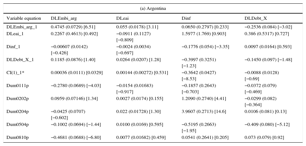
Finally as a fifth step, we test the CVAR model as a simultaneous equation system. Its results are summarized in Table 9a–g. We present the significance of the t-values for the different coefficients in order to highlight the differences between the countries18 – specifically, between dollarized and non-dollarized countries.
Econometric results.
| (a) Argentina | ||||
|---|---|---|---|---|
| Variable equation | DLEmbi_arg | DLeai | Dinf | DLDebt_X |
| DLEmbi_arg_1 | 0.4745 (0.0729) [6.51] | 0.055 (0.0178) [3.11] | 0.0650 (0.2797) [0.233] | −0.2536 (0.084) [−3.02] |
| DLeai_1 | 0.2267 (0.4613) [0.492] | −0.0911 (0.1127) [−0.809] | 1.5977 (1.769) [0.903] | 0.386 (0.5317) [0.727] |
| Dinf_1 | −0.00607 (0.0142) [−0.426] | −0.0024 (0.0034) [−0.697] | −0.1776 (0.054) [−3.35] | 0.0097 (0.0164) [0.593] |
| DLDebt_X_1 | 0.1185 (0.0876) [1.40] | 0.0264 (0.0207) [1.28] | −0.3997 (0.3251) [−1.23] | −0.1450 (0.097) [−1.48] |
| CI(1)_1* | 0.00036 (0.0111) [0.0329] | 0.00144 (0.00272) [0.531] | −0.3642 (0.0427) [−8.53] | −0.0088 (0.0128) [−0.69] |
| Dum0111p | −0.2780 (0.0689) [−4.03] | −0.0154 (0.01683) [−0.917] | −0.1857 (0.2643) [−0.703] | −0.0372 (0.079) [−0.469] |
| Dum0202p | 0.0959 (0.07146) [1.34] | 0.0027 (0.0174) [0.155] | 1.2090 (0.2740) [4.41] | −0.0299 (0.082) [−0.364] |
| Dum0204p | −0.0425 (0.0707) [−0.602] | 0.022 (0.01728) [1.30] | 3.9607 (0.2713) [14.6] | 0.0106 (0.081) [0.13] |
| Dum0504p | −0.1002 (0.0694) [−1.44] | 0.0100 (0.0169) [0.595] | −0.5195 (0.2663) [−1.95] | −0.409 (0.080) [−5.12] |
| Dum0810p | −0.4681 (0.0688) [−6.80] | 0.0077 (0.01682) [0.459] | 0.0541 (0.2641) [0.205] | 0.073 (0.079) [0.92] |
| (b) Brazil | ||||
|---|---|---|---|---|
| Variable equation | DLEmbi_br | DLii | Dinf | DLDebt__X |
| DLEmbi_br_1 | 0.2413 (0.0968) [2.49] | −0.3561 (0.1317) [−2.70] | −0.3595 (0.3619) [−0.993] | 0.6114 (0.2537) [2.41] |
| DLEmbi_br_2 | −0.0300 (0.0993) [−0.303] | 0.1743 (0.1352) [1.29] | −0.4834 (0.3714) [−1.30] | 0.1667 (0.2604) [0.640] |
| DLii_1 | 0.1173 (0.0988) [1.19] | −0.0219 (0.1345) [−0.163] | −1.206 (0.3696) [−3.26] | −0.7832 (0.2591) [−3.02] |
| DLii_2 | 0.0645 (0.0899) [0.718] | 0.4152 (0.1224) [3.39] | −0.3957 (0.3363) [−1.18] | −0.9867 (0.2358) [−4.19] |
| Dinf_1 | −0.0212 (0.0225) [−0.942] | −0.0352 (0.0307) [−1.15] | −0.2212 (0.0843) [−2.62] | 0.03738 (0.0591) [0.632] |
| Dinf_2 | 0.0392 (0.0208) [1.89] | −0.0917 (0.0282) [−3.25] | −0.1435 (0.0777) [−1.85] | 0.0879 (0.0545) [1.61] |
| DLDebt_X_1 | 0.0171 (0.0451) [0.379] | −0.0441 (0.0614) [−0.719] | −0.0632 (0.1688) [−0.375] | −0.4393 (0.1183) [−3.71] |
| DLDebt_X_2 | 0.0655 (0.0444) [1.48] | 0.0508 (0.0604) [0.841] | 0.0320 (0.1662) [0.193] | −0.2745 (0.1165) [−2.36] |
| CI(1)_1* | −0.0612 (0.074) [−0.819] | −0.4247 (0.1018) [−4.17] | 1.104 (0.2797) [3.95] | 0.6363 (0.1961) [3.25] |
| Dum0211p | 0.1891 (0.0453) [4.17] | −0.0553 (0.0617) [−0.898] | 1.1154 (0.1696) [6.58] | 0.2762 (0.1189) [2.32] |
| Dum0810p | −0.1312 (0.0433) [−3.03] | 0.0228 (0.0589) [0.387] | 0.0279 (0.1621) [0.172] | 0.0769 (0.1137) [0.677] |
| (c) Colombia | ||||
|---|---|---|---|---|
| Variable equation | DLEmbi_co | DLIMACO | Dinf | DLDebt_X |
| DLEmbi_co_1 | 0.1520 (0.095) [1.60] | 1.1126 (0.5134) [2.17] | −1.15585 (0.7058) [−1.64] | −0.4547 (0.3327) [−1.37] |
| DLIMACO_1 | −0.01669 (0.008016) [−2.08] | −0.5392 (0.0433) [−12.5] | 0.037718 (0.05953) [0.634] | −0.02614 (0.02806) [−0.932] |
| Dinf_1 | 0.01621 (0.01507) [1.08] | 0.1390 (0.06141) [1.71] | −0.184651 (0.1119) [−1.65] | −0.03471 (0.0527) [−0.658] |
| DLDebt_X_1 | 0.01487 (0.02810) [0.501] | −0.3494 (0.1518) [−2.30] | −0.097537 (0.2087) [−0.467] | −0.4635 (0.09839) [−4.71] |
| CI(1)_1* | −0.00061 (0.00306) [−0.202] | 0.1247 (0.01655) [7.54] | 0.03288 (0.02275) [1.45] | −0.005683 (0.01072) [−0.53] |
| Dum0405p | −0.1057 (0.02889) [−3.66] | 0.02470 (0.1561) [0.158] | 0.16086 (0.2145) [0.75] | 0.00572 (0.1011) [0.0566] |
| Dum0810p | −0.1548 (0.03011) [−5.14] | −0.3675 (0.1626) [−2.26] | 0.5895 (0.2236) [2.64] | 0.028015 (0.1054) [0.266] |
| Dum0901p | −0.00769 (0.030) [−0.255] | −0.8094 (0.1631) [−4.96] | −0.1852 (0.2243) [−0.826] | 0.1348 (0.1057) [1.28] |
| Dum0904p | 0.02359 (0.02929) [0.805] | −1.4419 (0.1582) [−9.11] | −0.02224 (0.2175) [−0.102] | 0.1485 (0.1025) [1.45] |
| Dum0907p | −0.01486 (0.03016) [−0.493] | −2.3418 (0.1629) [−14.4] | 0.15916 (0.2240) [0.711] | 0.00464 (0.1056) [0.0440] |
| (d) Chile | ||||
|---|---|---|---|---|
| Variable equation | DLEmbi_ch | DLipi | Dinf | DLDebt_X |
| DLEmbi_ch_1 | 0.2574 (0.0855) [3.01] | 0.2394 (0.1278) [1.87]** | −0.0509 (1.294) [−0.039] | −0.8188 (0.4075) [−2.01] |
| DLEmbi_ch_2 | −0.2627 (0.08522) [−3.08] | −0.077 (0.1274) [−0.611] | 3.3522 (1.29) [2.60] | −0.5122 (0.4061) [−1.26] |
| DLipi_1 | −0.04337 (0.06672) [−0.650] | −0.3102 (0.099) [−3.11] | −0.8168 (1.010) [−0.809] | 0.0184 (0.3179) [0.0582] |
| DLipi_2 | 0.0069 (0.0635) [0.109] | −0.02408 (0.09504) [−0.253] | −2.6025 (0.9622) [−2.70] | −0.153 (0.3030) [−0.508] |
| Dinf_1 | −0.0024 (0.0068) [−0.362] | −0.0049 (0.010) [−0.481] | −0.2602 (0.1042) [−2.50] | −0.054 (0.03281) [−1.65] |
| Dinf_2 | −0.001122 (0.0067) [−0.166] | 0.006 (0.01011) [0.665] | −0.3613 (0.1023) [−3.53] | −0.0704 (0.03222) [−2.19] |
| DLDebt_X_1 | −0.0069 (0.02465) [−0.280] | −0.0200 (0.0368) [−0.545] | −0.1078 (0.3731) [−0.289] | −0.6481 (0.1175) [−5.52] |
| DLDebt_X_2 | −0.0063 (0.0244) [−0.261] | 0.03496 (0.0364) [0.959] | −0.1842 (0.3692) [−0.499] | −0.3492 (0.1163) [−3.00] |
| CI(1)_1* | −0.007875 (0.0080) [−0.976] | 0.0018 (0.0120) [0.155] | 0.0939 (0.1222) [0.769] | −0.0318 (0.0384) [−0.829] |
| Dum0405p | −0.0995 (0.02314) [−4.30] | −0.0123 (0.0345) [−0.357] | 0.0668 (0.3502) [0.191] | −0.0393 (0.110) [−0.356] |
| Dum0810p | −0.1611 (0.02433) [−6.62] | −0.01164 (0.0363) [−0.320] | 0.0174 (0.3682) [0.0473] | 0.1631 (0.1159) [1.41] |
| Dum0901p | −0.0058 (0.02565) [−0.227] | −0.2303 (0.0383) [−6.01] | −0.5219 (0.3881) [−1.34] | 0.1623 (0.1222) [1.33] |
| (e) Mexico | ||||
|---|---|---|---|---|
| Variable equation | DLEmbi_mx | Diai | Dinf | DLDebt_X |
| DLEmbi_mx_1 | 0.1148 (0.0752) [1.53] | 0.9876 (11.12) [0.0888] | −3.0817 (1.039) [−2.97] | −0.5085 (0.3859) [−1.32] |
| DLEmbi_mx_2 | −0.4156 (0.0714) [−5.82] | 10.1342 (10.56) [0.960] | 0.8405 (0.9866) [0.852] | −0.4222 (0.3665) [−1.15] |
| DLEmbi_mx_3 | 0.0448 (0.0774) [0.580] | 29.4665 (11.45) [2.57] | −0.8210 (1.069) [−0.768] | −1.5534 (0.3973) [−3.91] |
| DLiai_1 | −0.0004 (0.0006) [−0.679] | −0.8000 (0.1026) [−7.80] | 0.0213 (0.0095) [2.22] | 0.0046 (0.0035) [1.30] |
| DLiai_2 | 0.0004 (0.0008) [0.602] | −0.5716 (0.1198) [−4.77] | 0.0207 (0.0111) [1.86] | 0.0027 (0.0041) [0.663] |
| DLiai_3 | 0.0001 (0.0006) [0.242] | −0.3033 (0.1031) [2.94] | 0.0079 (0.0096) [0.82] | −0.0017 (0.0035) [−0.486] |
| Dinf_1 | −0.0070 (0.0098) [−0.716] | 1.0485 (1.452) [0.722] | 0.3456 (0.1356) [2.55] [1.34] | −0.1244 (0.0503) [−2.47] |
| Dinf_2 | 0.0132 (0.0088) [1.49] | −0.9278 (1.315) [−0.706] | 0.2636 (0.1228) [2.15] | −0.0649 (0.0456) [−1.42] |
| Dinf_3 | 0.0017 (0.0070) [0.252] | 0.4255 (1.045) [0.407] | 0.2831 (0.0975) [2.90] | 0.0252 (0.0362) [0.696] |
| DLDebt_X_1 | −0.0080 (0.0203) [−0.393] | −4.9697 (3.009) [−1.65] | 0.2667 (0.2811) [0.949] | −0.2910 (0.1044) [−2.79] |
| DLDebt_X_2 | 0.0114 (0.0214) [0.533] | −6.9052 (3.165) [−2.18] | 1.3002 (0.2957) [4.40] | 0.0324 (0.1098) [0.296] |
| DLDebt_X_3 | 0.0293 (0.0214) [1.37] | −11.0014 (3.165) [−3.48] | 0.0677 (0.2957) [0.229] | 0.1342 (0.1099) [1.22] |
| CI(1)_1* | 0.0003 (0.0112) [0.0270] | 1.4923 (1.661) [0.898] | −0.9421 (0.1552) [−6.07] | 0.1206 (0.0576) [2.09] |
| Dum0810p | −0.1394 (0.0161) [−8.66] | −0.5771 (2.379) [−0.243] | 0.0734 (0.2223) [0.331] | −0.0255 (0.0825) [−0.309] |
| Dum0405p | −0.0605 (0.0164) [−3.68] | −2.3491 (2.431) [−0.966] | −0.1993 (0.2271) [−0.878] | −0.0531 (0.0843) [−0.630] |
| (f) Ecuador | ||||
|---|---|---|---|---|
| Variable equation | DLEmbi_ec | DLeai | Dinf | DLDebt_X |
| DLEmbi_ec_1 | 0.2528 (0.072) [3.50] | −0.086 (0.1061) [−0.819] | −0.0027 (0.0039) [−0.700] | −0.2698 (0.1149) [−2.35] |
| DLeai_1 | −0.031 (0.0604) [−0.527] | −0.6107 (0.088) [−6.88] | −0.0080 (0.0033) [−2.42] | 0.0937 (0.096) [0.0976] |
| Dinf_1 | 1.0619 (1.017) [1.04] | −0.1161 (1.493) [−0.077] | −0.1312 (0.055) [−2.35] | −1.504 (1.616) [−0.931] |
| DLDebt_X_1 | 0.125 (0.0613) [2.04] | −0.0820 (0.089) [−0.911] | 0.0009 (0.0033) [0.273] | −0.2481 (0.097) [−2.55] |
| CI(1)_1* | −0.6925 (1.073) [−0.645] | 0.0627 (1.575) [0.0399] | −0.4235 (0.059) [−7.17] | −0.7155 (1.705) [−0.42] |
| Dum0109p | 0.0125 (0.0569) [0.221] | 0.0596 (0.083) [0.714] | 0.013 (0.0031) [4.22] | −0.089 (0.09) [−0.987] |
| Dum0301p | 0.083 (0.056) [1.46] | 0.0077 (0.083) [0.0931] | 0.017 (0.0031) [5.43] | 0.0109 (0.09) [0.121] |
| Dum0810p | −0.4618 (0.058) [−7.93] | −0.1432 (0.0854) [−1.68] | −0.0047 (0.0032) [−1.49] | 0.200 (0.092) [2.16] |
| Dum0811p | −0.4984 (0.065) [−7.62] | −0.0083 (0.096) [−0.08] | −0.0071 (0.0035) [−1.97] | 0.0721 (0.1039) [0.69] |
| Dum0906p | 0.1389 (0.056) [2.46] | −0.0377 (0.082) [−0.455] | −0.0007 (0.0031) [−0.257] | −0.410 (0.089) [−4.92] |
| (g) Panama | ||||
|---|---|---|---|---|
| Variable equation | DLEmbi_pa | DLrev_c | Dinf | DLDebt_X |
| DLEmbi_pa_1 | 0.2995 (0.074) [4.00] | 0.04671 (0.1630) [0.287] | 3.8661 (1.595) [2.42] | −0.4881 (0.6171) [−0.791] |
| DLrev_c_1 | −0.0387 (0.0456) [−0.849] | −0.1722 (0.0992) [−1.74] | 0.7122 (0.9714) [0.733] | 0.1170 (0.3757) [0.311] |
| Dinf_1 | −0.0058 (0.0043) [−1.33] | −0.0228 (0.0095) [−2.40] | −0.2284 (0.093) [−2.45] | 0.0769 (0.036) [2.14] |
| DLDebt_X_1 | −0.00147 (0.01302) [−0.113] | 0.0337 (0.02832) [1.19] | 0.6640 (0.2772) [2.40] | −0.0085 (0.1072) [−0.919] |
| CI(1)_1* | −0.0988 (0.028) [−3.51] | 0.1816 (0.0612) [2.97] | −0.0633 (0.5992) [−0.106] | −0.1927 (0.2318) [−0.832] |
| CI(2)_1* | 0.0067 (0.0092) [0.737] | 0.00694 (0.0200) [0.346] | −0.9952 (0.1964) [−5.07] | −0.2118 (0.0759) [−2.79] |
| Dum0401p | 0.02503 (0.02011) [1.25] | −0.00535 (0.0437) [−0.122] | −1.9271 (0.4283) [−4.50] | 0.3987 (0.1656) [2.41] |
| Dum0810p | −0.1819 (0.0202) [−8.99] | 0.0221 (0.044) [0.0502] | −0.4506 (0.4310) [−1.05] | 0.1666 (0.1667) [1.00] |
Notes: Std-errors are in parenthesis and t-values in brackets. *Argentina: CI(1)=Inf.
Notes: Std-errors are in parenthesis and t-values in brackets.*Brazil: CI(1)=Lii - 0.18221*Inf+0.1918*LDebt_X.
Notes: Std-errors are in parentheses and t-values in brackets. *Colombia: CI(1)=LEMBI_co – 1.0232*LIMACO – 2.4449*Inf.
Notes: Std-errors are in parentheses and t-values in brackets. *Chile: C(1)=LEMBI_ch+0.07898*LDebt_X – 0.2549*Inf. **When non-significant dummies were excluded this coefficient becomes significant.
Notes: Std-errors are in parentheses and t-values in brackets. *Mexico: C(1)=Inf.
Notes: Std-errors are in parentheses and t-values in brackets. *Ecuador: CI(1)=Inf_1.
Notes: Std-errors are in parentheses and t-values in brackets. *Panama: CI(1)=-0.79176*Lrev_c+LEmbi_pana and CI(2)=0.61532*Inf+LDebt_X – 0.44483*LRev_c.
As mentioned, the results of the parameter estimations that describe the short run effects over variables are presented in Table 9a–g. Specifically, Table 9a–e correspond to non-dollarized countries and Table 9f and g to the dollarized ones (Ecuador and Panama). In these tables, the presence of t-values makes it easy to distinguish between significant and non-significant coefficients across the seven emerging countries in the sample.
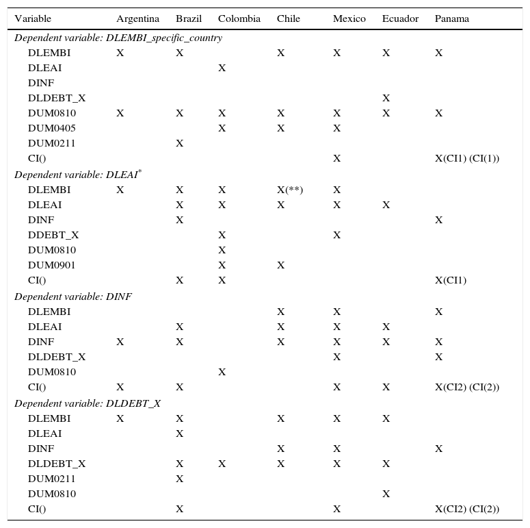
Table 10 presents the comparative analysis of the seven emerging countries.
Comparative analysis taking only the significant coefficients into account.
| Variable | Argentina | Brazil | Colombia | Chile | Mexico | Ecuador | Panama |
|---|---|---|---|---|---|---|---|
| Dependent variable: DLEMBI_specific_country | |||||||
| DLEMBI | X | X | X | X | X | X | |
| DLEAI | X | ||||||
| DINF | |||||||
| DLDEBT_X | X | ||||||
| DUM0810 | X | X | X | X | X | X | X |
| DUM0405 | X | X | X | ||||
| DUM0211 | X | ||||||
| CI() | X | X(CI1) (CI(1)) | |||||
| Dependent variable: DLEAI* | |||||||
| DLEMBI | X | X | X | X(**) | X | ||
| DLEAI | X | X | X | X | X | ||
| DINF | X | X | |||||
| DDEBT_X | X | X | |||||
| DUM0810 | X | ||||||
| DUM0901 | X | X | |||||
| CI() | X | X | X(CI1) | ||||
| Dependent variable: DINF | |||||||
| DLEMBI | X | X | X | ||||
| DLEAI | X | X | X | X | |||
| DINF | X | X | X | X | X | X | |
| DLDEBT_X | X | X | |||||
| DUM0810 | X | ||||||
| CI() | X | X | X | X | X(CI2) (CI(2)) | ||
| Dependent variable: DLDEBT_X | |||||||
| DLEMBI | X | X | X | X | X | ||
| DLEAI | X | ||||||
| DINF | X | X | X | ||||
| DLDEBT_X | X | X | X | X | X | ||
| DUM0211 | X | ||||||
| DUM0810 | X | ||||||
| CI() | X | X | X(CI2) (CI(2)) | ||||
Note: The results shown are the ones obtained when non-significant dummies were eliminated. CI(): Specifies only the variables included in each long run relationship, which are described in Table 8. *This variable changes depending on the country (see Table 4). **When non-significant dummies were excluded this coefficient becomes significant.
Looking across the columns in Table 9a–g, the following conclusions can be drawn: (1) The Emerging Bond Market Index (EMBI) is generally affected by global factors (proxied by dum0810p which captures the beginning of the financial crisis) and their own shocks, since all the countries in the sample, except Colombia, have a significant lagged DLEMBI coefficient in their EMBI equations. Debt_x does not seem to be relevant for explaining the EMBI behaviour, unless a country has defaulted on its debt obligations (as Ecuador did); (2) Economic activity is affected by the EMBI in all countries but dollarized ones; which represents the first important finding of this study, suggesting that in non-dollarized countries, debt-servicing costs may have an important impact on the evolution of the economy; (3) In most cases, inflation follows a long run relationship. In our opinion, this is the second important finding of this research, since it means that a country does not need to be dollarized to reach stable inflation levels. Inflation targeting might be behind the non-dollarized countries’ results19; (4) In general, investors look at the evolution of the EMBI to make their next decisions regarding sovereign bond debt investment. Colombia and Panama are the exceptions; (5) In general, the EMBI does not follow a long run relationship (with the exception of Mexico and Panama). (6) Finally, it seems that contagion effects are present in only three countries: Colombia, Chile, and Mexico. These inter-relationships are captured by dum0405p and dum0901p variables. The former affects the EMBI in the three countries, whilst the latter affects the economic activity in just the first two countries.
5ConclusionsThe two main findings of this paper are: (i) economic activity is affected by the EMBI in all the countries except the dollarized ones; and (ii) inflation follows a long run relationship for most of the sample (the exceptions being Colombia and Chile), showing that a country does not need to be dollarized to achieve a stable inflation level. Our results suggest that in Latin America countries the pricing of risk (EMBI) depends mostly on global factors. Nevertheless, its evolution affects foreign lenders’ prospective debt investments, as well as domestic economic activity, except in dollarized countries.
These results may suggest the following conclusions. First, dollarization may ensure that currency mismatches will not occur during domestic economic crises; thus, the EMBI is more stable and these countries’ access to debt markets is easier due to their lower vulnerability to EMBI shocks. Second, dollarized countries are not as dependent on international reserves (they use the US dollar both to develop their economies and to pay their debts), as their non-dollarized counterparts which need international reserves to pay their debts but use national currencies to develop their economies. This comparative analysis between two dollarized and five non-dollarized countries suggests that dollarization may isolate the evolution of the broadest emerging market debt benchmark, the EMBI. These results are particularly interesting since there are some non-dollarized Latin American countries which are already doing (relatively) well on their own. We think that they should encourage fiscal discipline in order to avoid a debt crisis situation since, in a default context, due to the interrelationship between their economic activity and the EMBI evolution; they would face much more trouble than dollarized economies.
Besides, our results also suggest that in the long run, non-dollarized countries with inflation targeting policies achieve similar levels of inflation to those obtained by their dollarized counterparts. This result is consistent with those presented by other authors (Bernanke and Mishkin, 1997; Bernanke et al., 1999). The novelty is to reach this conclusion by means of the cointegrated VAR approach which identifies long-run relationships, including a stationary inflation variable in non-dollarized countries.
Financial support from Spanish Ministry of Economy and Competitiveness through grant ECO2016-76203 and through Plan Estatal de Investigación Científica y Técnica y de Innovación is gratefully acknowledged. The authors would like to thank Katarina Juselius for their useful and interesting comments and suggestions.
Financial support from Spanish Ministry of Economy and Competitiveness through grant ECO2016-76203 and through Plan Estatal de Investigación Científica y Técnica y de Innovación is gratefully acknowledged. The authors would like to thank Katarina Juselius for their useful and interesting comments and suggestions.
The results are not conclusive, though. Whilst Krugman (2013) shows how Eurozone members have had more trouble managing their debts than countries outside it, Rose (2013) suggests that the exchange rate regime does not matter.
The JP Morgan Emerging Markets Bonds Index Global tracks total returns for traded external debt instruments in emerging markets. The EMBI Global includes US dollar-denominated Brady bonds, loans, and Eurobonds with an outstanding face value of at least $500 million. Daily historical index levels have been reported since December 31, 1993. See Morgan (1999) for more details.
Country risk refers to the likelihood that a sovereign state (borrower) may be unable and/or unwilling to meet its obligations towards foreign lenders and/or investors (Krayenbuehl, 1985).
The literature on country risk is essentially four decades old. The two pioneering articles were published by Frank and Cline (1971) and Feder and Just (1977). Since then, authors have attempted to establish the determinants and the econometric criteria to estimate, evaluate, and forecast country risk in different economies.
In financial jargon, the investors’ degree of risk aversion is usually called “investor appetite for risk”.
See Hoti and McAller (2004) and Maltritz and Molchanov (2013), which present a summary of the explanatory variables and econometric models used in previously published empirical articles.
The Economic Activity Index for Argentina, Ecuador and Colombia is presented as the monthly proxy of GDP by their respective National Statistic Institutes. In the case of Mexico we use the Industrial Activity Index instead of the Global Economic Activity Index because the latter, not only does not include all the sectors of the economy, but also is still a preliminary variable that is being adjusted by private and public enterprises over time. Indeed, in Mexico, the Industrial Index has historically been used as a proxy of GDP because their strong co-movements (OECD, 2012). Brazil and Chile models include the Industrial Index as well, but this time the reason is data availability constraint.
This section relies heavily on Juselius (2006).
In April 1991 the Convertibility Plan was launched, which pegged the peso 1-to-1 to the US dollar. This plan was replaced with a dual exchange rate regime based on an official exchange rate of 1.4 pesos per dollar for public sector and tradable transactions, while other transactions were conducted at market rates. By June 2002 the exchange rate reached 4 pesos per dollar (Kaminsky et al., 2009; Mourelle, 2010).
See Hornbeck (2013).
In June 2009 the Correa government defaulted on $3.2 billion of foreign public debt, and then completed a buyback of 91 per cent of the defaulted bonds (Sandoval and Weisbrot, 2009).
Inflation only achieved a stable level in Ecuador after the first quarter of 2003.
Several articles have presented empirical evidence of contagion effects within these countries. For instance, based on the estimation of a multivariate regression model, Mathur et al. (2002) conclude that there were spillover contagion effects from the Mexican market to the Chilean market during the 1994 peso crisis. Moreover, Kaminsky and Schmukler (2001) study whether capital controls affect the link between domestic and foreign stock market prices and interest rates, and find that equity prices are more internationally linked than interest rates.
McGuire and Schrijvers (2003) find high correlations of common factors with S&P500, US Treasury yield curve and oil prices.
On the supply side, when Treasury bond rates go up, the increased debt servicing cost decreases the supply of US external debt. This in turn increases the price of emerging bonds averaged by the EMBI.
The first four steps were performed using the software CATS. Recursive estimation to check parameters stability is available under request.
This econometric work was carried out with the software Ox Metrics.
Corbo and Schmidt-Hebbel (2001) analyze the experience of Latin America countries with inflation targeting regimes and classify Brazil and Chile as full-fledged inflation targeting, whilst Colombia and Mexico are classified as partial inflation targeting regimes. These authors emphasize the substantial progress of these countries to achieve low one digit inflation levels without output sacrifices.