


The aim of statistical inference is to predict the parameters of a population, based on a sample of data.
Inferential statistics encompasses the estimation of parameters and model predictions.
The present article describes the hypothesis tests or statistical significance tests most commonly used in healthcare research.
The basis of statistical inference is to determine (infer) an unknown parameter for a given population, based on a sample or subset of individuals belonging to the mentioned population, and fundamented upon the frequency interpretation concept of probability. Basically, the aspects studied by inference statistics are divided into estimation and hypothesis testing.1
The quest for new knowledge in healthcare generates clinico-epidemiological hypotheses that constitute tentative declarations in reference to the causal relationship between exposure and disease.2
On carrying out an observational or experimental study, the existence of a genuine effect is assumed, underlying exposure or treatment, and which the epidemiological study can only estimate. Investigators use statistical methods to determine the true effect of the results of their studies. Since the 50s, the paradigm of statistical inference has been statistical significance testing or hypothesis testing, based on the generalisation of a hybrid between two methods of opposite origin: the method for measurement of the degree of incompatibility of a set of data, developed by Ronald Fisher, and the hypothesis selection procedure, developed by Jerzy Neyman and Egon Pearson in the period 1920–1940.3 The start of any type of research is based on the formulation of the corresponding “null hypothesis” (H0), representing the hypothesis to be evaluated and possibly rejected. The null hypothesis is commonly defined by the null existence of differences between the results of the comparator groups, and H0 in turn is the contraposition to the so-called alternative hypothesis (H1).
DefinitionsType of hypothesisDepending on the hypothesis established, hypothesis test used can be bilateral or unilateral. Contrasting is bilateral (also known as two-tailed contrasting) when the inequality expressed by the alternative hypothesis can manifest in either sense. Contrasting in turn is unilateral (or single-tailed) when rejection of the null hypothesis can only occur in one given sense – with distinction between right (<) and left (>) unilateral contrasting. Based on the evidence of previous studies, the investigator must establish whether the hypothesis poses a unilateral or bilateral scenario.4
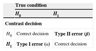
When accepting or rejecting a hypothesis test, we have no absolute certainty that the decision taken is correct in the population. It is necessary to evaluate such certainty based on: I) significance level (α), i.e., the value quantifying the error made on accepting H1 when H0 is actually true in the population. This is referred to as type I error, pre-established in the form of acceptance-rejection thresholds of 1%, 5% or 10%, depending on the type of investigation involved. II) If H0 is accepted when H1 is actually true in the population, the error is referred to as type II error (β). The power of a test is defined as 1−β and indicates the probability of accepting H1, i.e., the capacity to detect alternative hypotheses5 (Table 1).
Contrast decisionOn carrying out a hypothesis test, we must take a decision regarding a “true situation” based on the calculations made with a representative sample of data. The accepted standard level of significance is α=0.05, i.e., the probability of error on rejecting H0 when the latter is actually true, must be no more than 5%. In deciding whether to accept or reject H0, we obtain a p-value as a result of the contrast made; since this value is a probability, it ranges between 0 and 1. This probability is defined as the minimum level of significance with which H0 is rejected. The value is compared with the level of significance; as a result, if the p-value is lower than the level of significance considered (p<0.05), we will have enough sample evidence to reject the contrasted null hypothesis in favour of the alternative hypothesis.
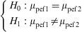
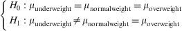
As an example, in a retrospective cohort study attempting to determine whether there is an increased prevalence of asthma in children who were not breastfed until four months of age (bf4-) versus a group of infants breastfed until four months of age (bf4+), the following hypothesis test was made, with an established significance level of α<0.05:
H0: %asthma (bf4−)=%asthma (bf4+), i.e., the null hypothesis is established as the equality of asthma prevalence in the population with and without maternal lactation for over four months (α>0.05).
H1: %asthma (bf4−)≠%asthma (bf4+), i.e., there are differences in asthma prevalence between the population with and without maternal lactation for over four months (α<0.05).
Type of variablesDepending on the kind of variables to be contrasted, we select one hypothesis test or another as the most appropriate. If the variables are quantitative, i.e., they can be expressed numerically, use is made of one type of test. In turn, the alternative type of test is used in the case of qualitative variables, i.e., referred to non-measurable properties of the study subjects, of an ordinal or nominal nature.6
Type of samplesIn order to compare two or more populations we must select a sample of each one. In this sense two basic types of samples are identified: dependent and independent samples. The type of sample in turn is determined by the sources used to obtain the data.
Dependent series are established when one same information is evaluated more than once in each subject of the sample, as occurs in pre-post study designs. Likewise, paired observations can be found in case-control studies when the cases are individually paired with one or several controls. When two sets of unrelated sources are used – one for each population – independent sampling is established.7
NormalityThe normal or Gaussian distribution is the most important continuous distribution in biostatistics, since many of the statistics used in testing hypothesis are based on the normal distribution. This distribution is encompassed within the central limit theorem, which constitutes one of the fundamental principles in statistics. It indicates that for any random variable, on extracting samples with a size of n>30, and on calculating the sample means, the latter will be seen to show a normal distribution. The mean will be the same as that of the variable of interest, and the standard deviation of the sample mean will be approximately the standard error.8
The normal distribution shows the following properties:
- I)
It is a continuous function asymptotically tending towards infinity at both extremes.
- II)
It is symmetrical with respect to the mean, i.e., 50% of the observed values will be above or below the mean.
- III)
The mean, median, and mode take the same value.
Together with the description of the mean and standard deviation, a visual inspection is recommended of the distribution of the samples capable of suggesting normality, based on histograms. In addition, it is essential to use the normality tests, which are applied to check that the data set effectively follows a normal distribution. Checking the normality hypothesis is an essential prior step to select the hypothesis test in a correct way.9
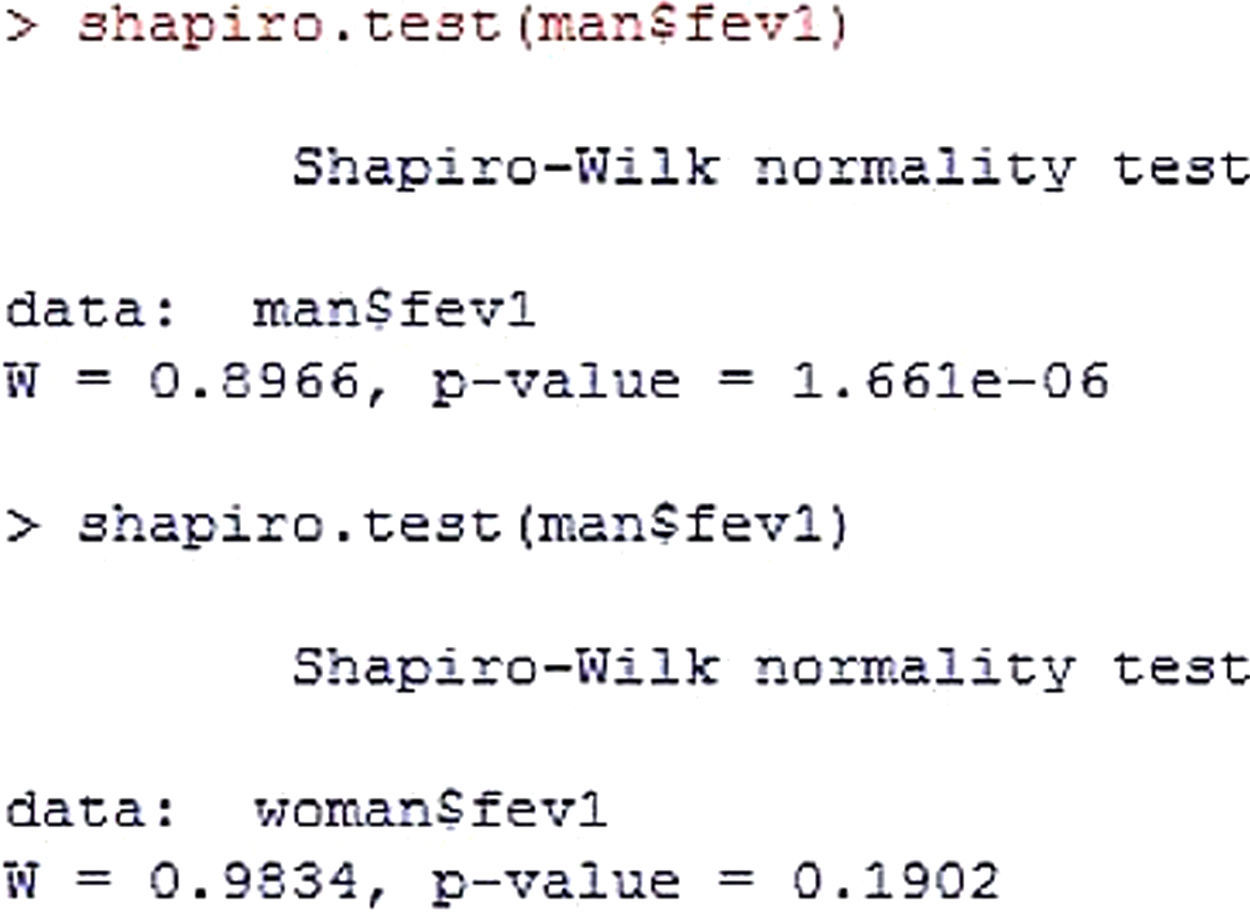
The tests used for checking the normality hypothesis are the Kolmogorov-Smirnoff and Shapiro-Wilks tests - the null hypothesis being that the data set is similar to the normal distribution. Accordingly, in the event of rejecting H0, the study distributions will be non-normal.Example 1 Forced expiratory volume (fev) is recorded in allergic children. The normality of the variable is then studied in the groups formed by gender.
Hypothesis test
Note that significance in the men group is less than 0.05 (Figure 1), while the variable shows a normal distribution in the women group. Since the men group shows a non-normal distribution, it is concluded that normality of the study variable is not met. In this case the alternative hypothesis (H1) would be accepted.Homogeneity of variances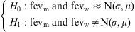

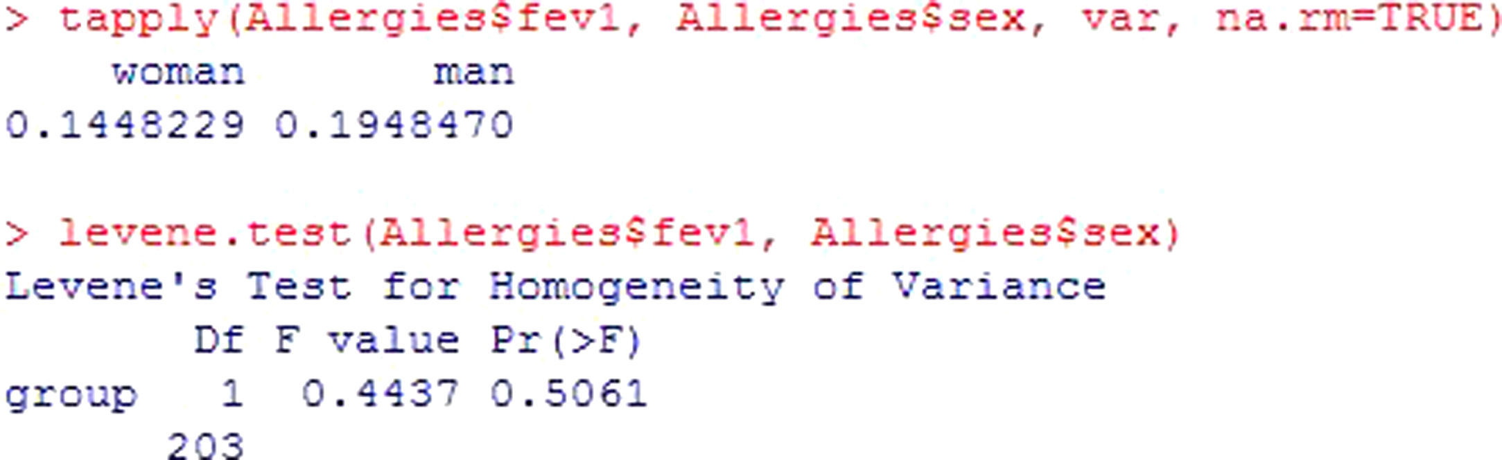
A second criterion for using parametric tests is that the variances of the distribution of the quantitative variable in the populations from which the comparator groups originate must be homogeneous. The Levene test is used to check the homogeneity of variances – the null hypothesis of the test being that the variances are equal.Example 2 Continuing with the previous example, the homogeneity of variances of forced expiratory volume in the two groups is studied.
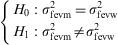
Once the variances of the groups have been presented, the statistic and its significance are shown. Since p>0.05, it is assumed that there are no differences in variance per group, and the null hypothesis of the test is not rejected. Figure 2.
Type of test¿
If we assume normality and homoscedasticity of the study variables, use is made of the parametric tests. These tests involve a certain probability distribution of data – the most common being those based on the normal probability distribution.
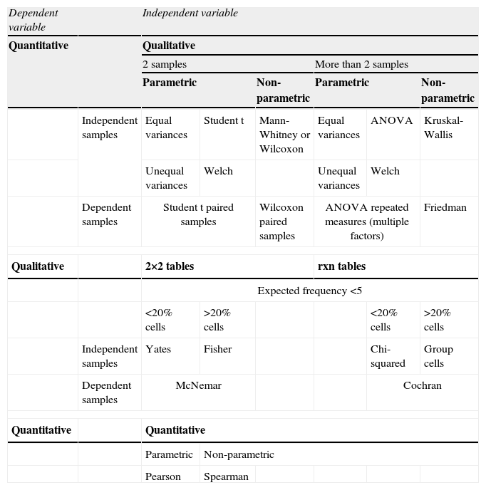
If the variables to be contrasted fail to meet some of the abovementioned criteria, use is made of the non-parametric tests – these being tests that do not assume a certain probability distribution of the data (hence their description also as free distribution tests). These tests are based only on ordering and counting procedures – the central tendency parameter being the median. Whenever the normality and homogeneity of variance criteria are met, use must be made of the parametric tests, since they offer greater power-efficiency performance than the non-parametric tests.10 A summary of the different types of contrasts can be found in Table 2.
Summary of the different types of hypothesis test.
| Dependent variable | Independent variable | ||||||
| Quantitative | Qualitative | ||||||
| 2 samples | More than 2 samples | ||||||
| Parametric | Non-parametric | Parametric | Non-parametric | ||||
| Independent samples | Equal variances | Student t | Mann-Whitney or Wilcoxon | Equal variances | ANOVA | Kruskal-Wallis | |
| Unequal variances | Welch | Unequal variances | Welch | ||||
| Dependent samples | Student t paired samples | Wilcoxon paired samples | ANOVA repeated measures (multiple factors) | Friedman | |||
| Qualitative | 2×2 tables | rxn tables | |||||
| Expected frequency <5 | |||||||
| <20% cells | >20% cells | <20% cells | >20% cells | ||||
| Independent samples | Yates | Fisher | Chi-squared | Group cells | |||
| Dependent samples | McNemar | Cochran | |||||
| Quantitative | Quantitative | ||||||
| Parametric | Non-parametric | ||||||
| Pearson | Spearman | ||||||
On comparing the equality or difference between two groups through a quantitative measure, for example, the concentration of pollen in two different populations, we generally use the Student's t-test for independent samples. The null hypothesis of the test in this case would be the equality of means versus the alternative hypothesis of differences between the means.

The conditions for application of this test are:
- •
The contrasted variable is quantitative.
- •
The two groups are independent.
- •
The normality hypothesis must be satisfied in both groups, or else the sample size must be large (n>30) in both groups of subjects.
- •
The variances of the groups must be equal.
In checking normality and equality of variances, use is made of the Shapiro-Wilks and Levene tests, respectively, commented above (Examples 1 and 2).
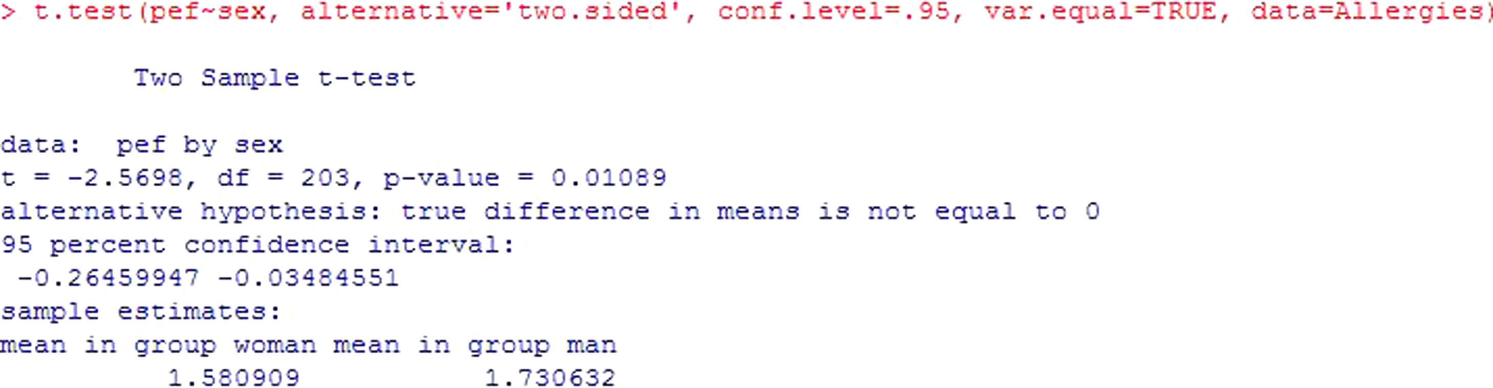
Example: An evaluation is made of possible differences in peak expiratory flow (pef) between groups formed by gender. In this case the independent groups are formed by males and females – the variable being recorded as pefm and pefw respectively.
The hypothesis test would be:
or, equivalently: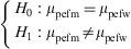
Using the R commander program for the calculations, and assuming that there are more than 30 cases per group, we obtain this output (Figure 3). After checking the equality of variances, use is made of the Student's t-test for independent samples (if equality of variance is not confirmed, the program corrects the situation with the Welch test). The result of the contrast yields a value p=0.01*, which makes it possible to reject the null hypothesis of equality of means, and thus affirm that the mean pef values are different for boys and girls. The output also shows the confidence interval for the difference of means [−0.264, −0.035], which in this case does not contain zero – thus confirming rejection of the null hypothesis. Lastly, it shows the means of the variable pef for both groups.

* Note: For all the results, when the p values are very small, we round to p<0.001. Likewise, the number of decimal points shown for all the results will be the same.
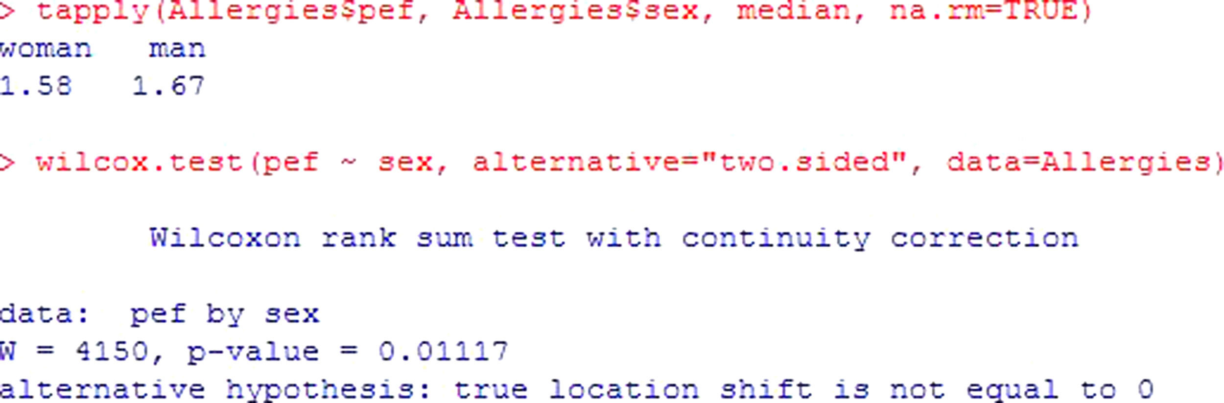
In the event that the normality hypothesis is not satisfied, and if the sample size is small (n<30), a non-parametric test should be used. In this case we apply the Mann-Whitney or Wilcoxon test for two samples.
Example: Considering the same example as before, and assuming non-normality of the variables, see Figure 4. The interpretation is the same as for the previous test, yielding a value p<0.05; the registered fev values differ by gender in a statistically significant way, with important higher values in males.
Testing two related samples (paired data)
In the case of dependence between the groups to be compared, the required test is different. This situation can be found for example when using as groups the same subjects but at different moments in time. An example would be the comparison of peak expiratory flow in a group of patients at the start of treatment and again three months later.
Assuming a sample size n>30 in both groups, we use the Student's t-test for paired samples.
The applicability conditions are the same as in the previous case, except as regards the independence of the groups.
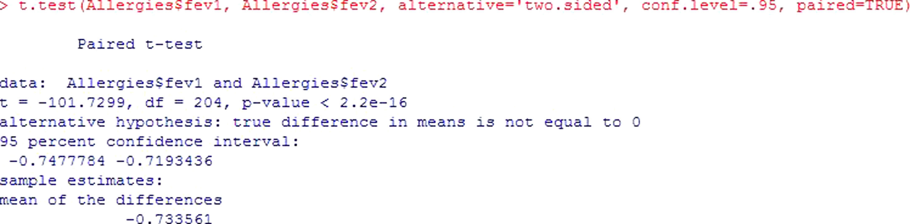
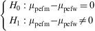
Example: An evaluation is made of the peak expiratory flow (pef1) values measured in children with asthma. After the application of treatment, patients are subjected to follow-up, and the study variable is again measured five weeks later (pef2), to determine whether the change induced by treatment is significant or not.
The contrast to be made would be the following:
In this case, the p-value shows that the difference in pef levels at the two measurement timepoints is statistically significant (p<2.2e-16). Figure 5. Since the difference of means is negative, it is shown that treatment intervention reduces fev values in the patients.In the same way that test for independent samples, the confidence interval does not contain zero – thus confirming the hypothesis that means are different.

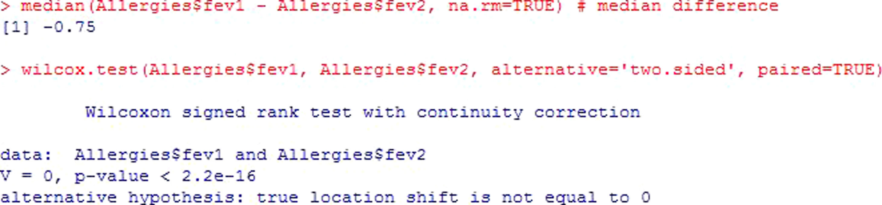
The non-parametric version of this test is the Wilcoxon rank test.
The previous example is shown, applying the corresponding non-parametric test for the case of dependent or paired samples. Figure 6.
Testing more than two samples
Up to this point we have seen the tests used to contrast numerical variables between two groups formed by categories of a character type variable. The Student's t-test is the appropriate instrument for testing this hypothesis, though the limitation that the number of groups is limited to two.
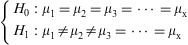
When there are more than two groups, the analysis of variance (ANOVA) must be applied. The null hypothesis of the test in this case would be equality of all the means, while the alternative hypothesis would be that some of them are different (not all means, but at least one mean value).
The applicability conditions of this test son:
- •
The contrasted variable is quantitative.
- •
The compared groups are independent.
- •
The normality hypothesis must be satisfied in all of the groups, or else the sample size must be large (n>30) in all of them.
- •
The variances must be equal in all the groups.
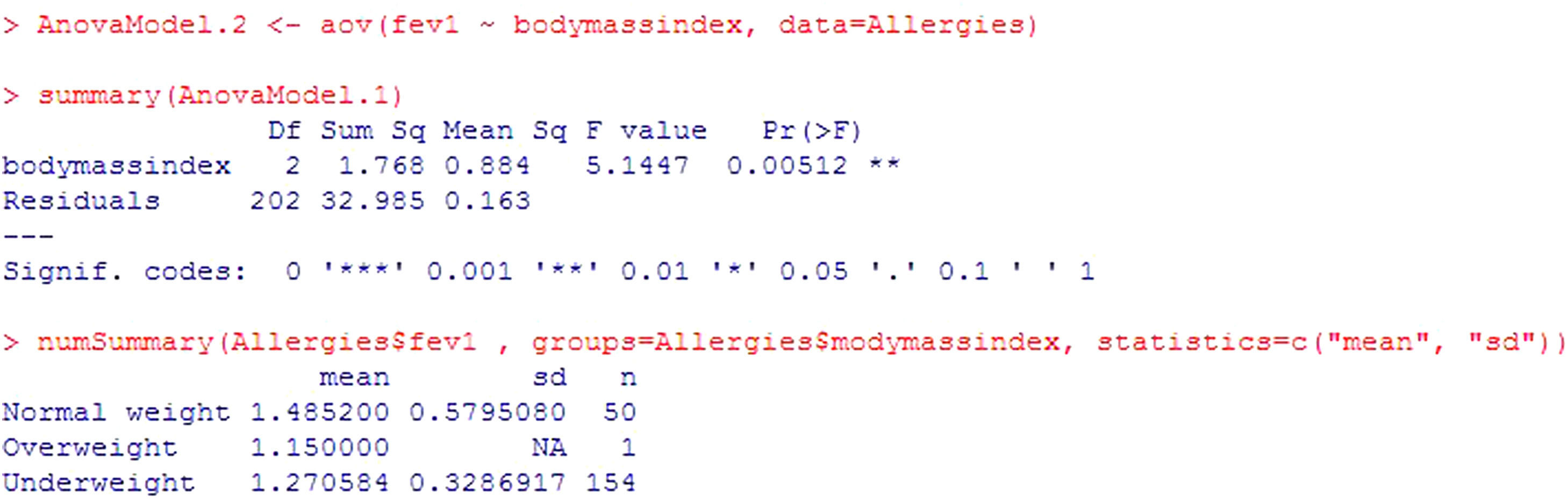
Example: A study is made to determine whether fev is related to child body weight. To this effect use is made of the body mass index variable (BMI), categorized as low weight, normal weight and overweight.
The program output (Figure 7) reports the mean and standard deviation of the variable to be contrasted in each category of body mass index variable. Clear differences are seen in the means of different groups, and in addition the p-value=0.00512. It is thus concluded that there are statistically significant differences. Patients with normal body weight are seen to have significantly higher fev values than low weight patients.

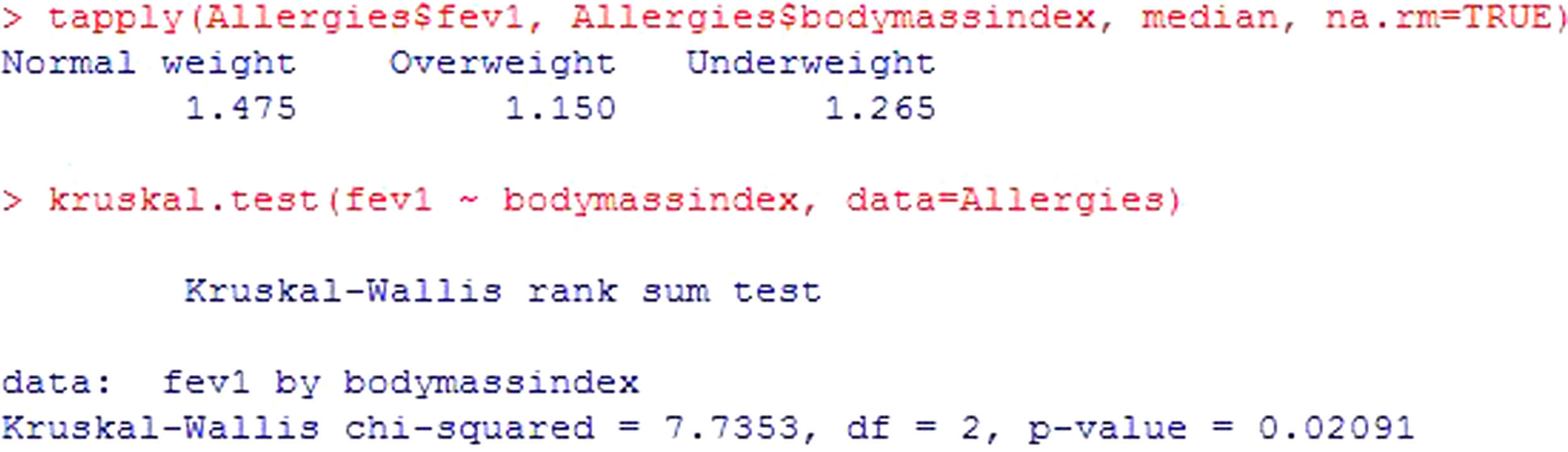
In the same way as in the rest of contrasts seen up to this point, there is a non-parametric version of the ANOVA test, for application in the case where the hypothesis of the model is not verified: the Kruskal Wallis test. For these same data, and assuming non-normality, see Figure 8. As in the previous case, significant differences are described (p=0.02) - the forced expiratory volume values in the patients with normal body weight being significantly greater.
Testing more than two related samples
The data independence hypothesis may be breached in certain cases, such as for example when repeated measurements are made over time. In this case the test to be used is ANOVA but in its version for related data, i.e., multiple factors ANOVA.
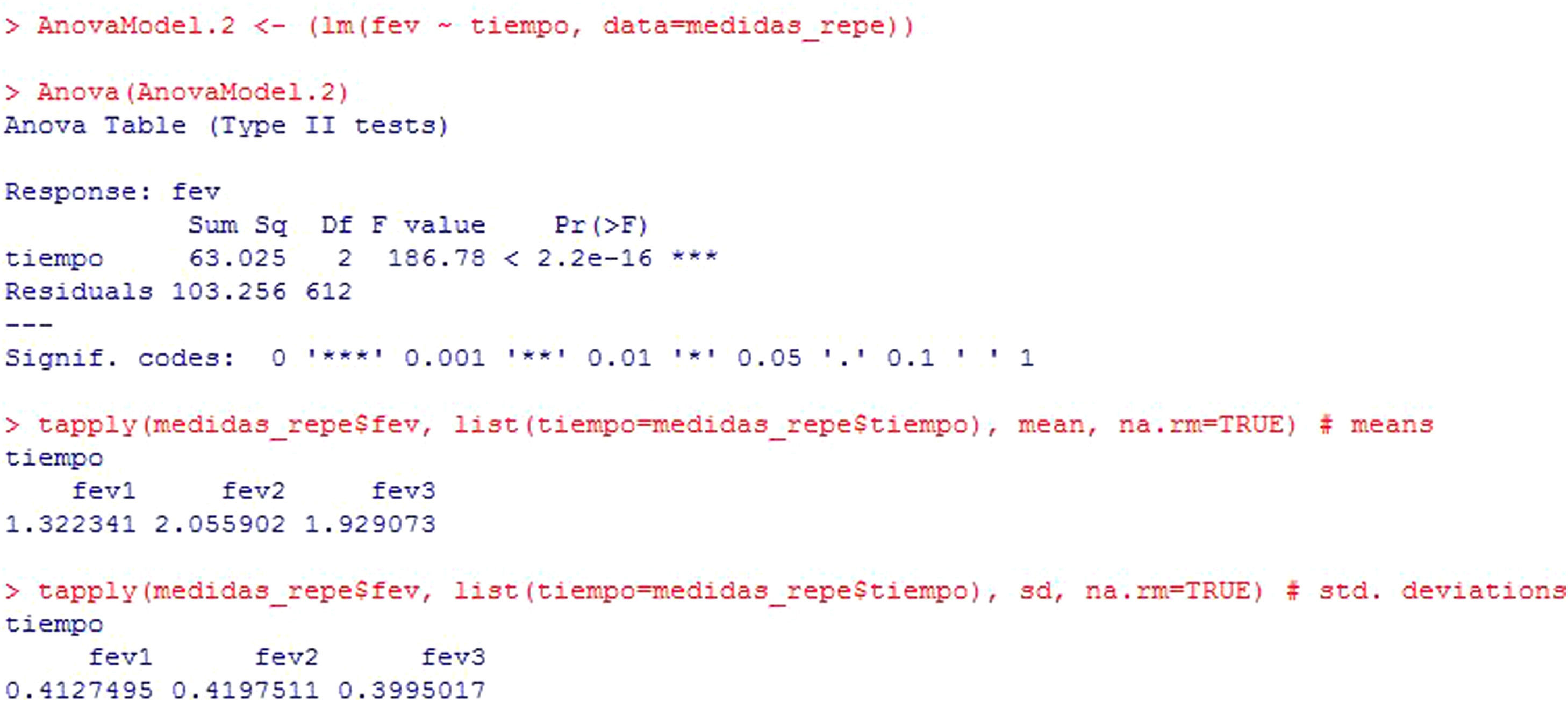
Example: A treatment for asthma is applied in children, with the measurement of fev initially (fev1), after one month of treatment (fev2) and three months later (fev3). Results are compared with a repeated measures test, since these are the same children in which one same variable is measured at different points in time.
To determine whether the change produced by the treatment is statistically significant, the test to be made would be:
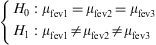
In this example (Figure 9), the result shows that there are statistically significant differences among the three measurements of fev (p<2.2e-16). In addition, the program reports the mean and standard deviation for the variable at the three timepoints, where these differences are already manifest.

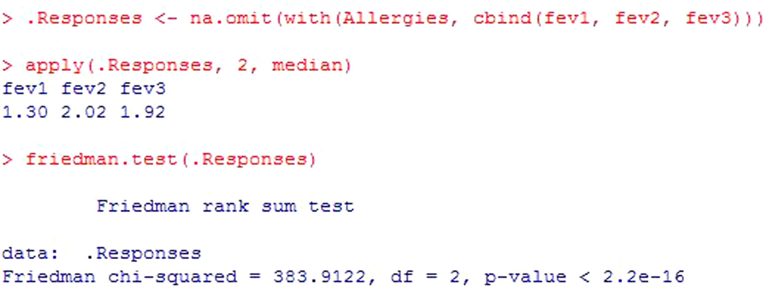
The Friedman rank sum test is the test to be used in those cases which do not comply with the normality hypothesis and the sample size is small. For the same data as in the previous example, see Figure 10.
Testing correlation between two independent variables
The possible association between two numerical variables, for example, the forced expiratory volume (fev) and peak expiratory flow (pef), constitutes a correlation.
This correlation indicates whether a change in fev modifies the corresponding pef value. It may be positive (or direct) when an increase in patient fev is in turn associated with an increase in pef. In turn, a negative (or indirect) correlation is observed when an increase in one of the variables results in a decrease in the other.
Based on the principle that the null hypothesis always refers to equality, the contrast of hypothesis ascribed to the question above would be as follows:
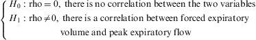
The statistics used for testing this hypothesis are the Pearson or Spearman tests.
The conditions for applying these statistics are that both variables must be numerical and the sample independent.
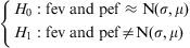
In the same way as in other contrasts in which numerical variables are used, the normality hypothesis must be satisfied. In this case there are two numerical variables, as a result of which both must meet this condition (H0: fev and pef≈N(σ, μ)) in order to apply a parametric test – in this case the Pearson test – or alternatively the sample size must be large (n≥30). In the event that some variable fails to meet the normality criterion and/or the sample size is under 30 (the criterion being left to the investigator or to the norms of the journal in the case of a study for publication), application is made of the Spearman test.
Example: Based on a database of allergic patients, a study is made to determine whether there is a relationship between the forced expiratory volume (fev) of the patients and their peak expiratory flow (pef), i.e., the aim is to determine whether changes in fev imply changes in pef. The contrast to be made would be the following:
Applicability conditions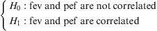
- •
The variables entered in the contrast are numerical within an independent sample.
- •
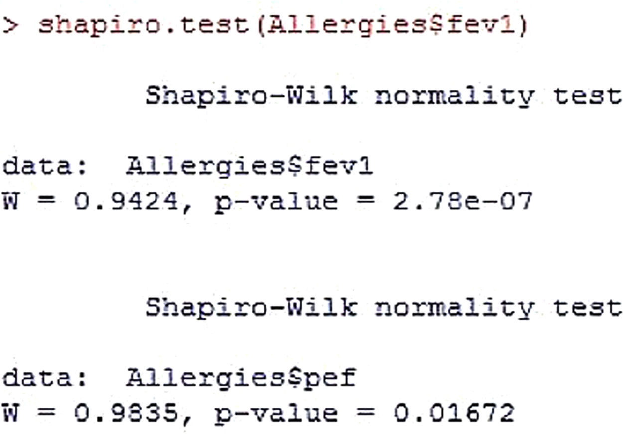
Normality
In both variables significance is less than 0.05; as a result, it is concluded that normality is not met in either of the two. The alternative hypothesis, H1, would thus be accepted (Figure 11).

Therefore, for this condition, the test to be used would be the Spearman non-parametric test.
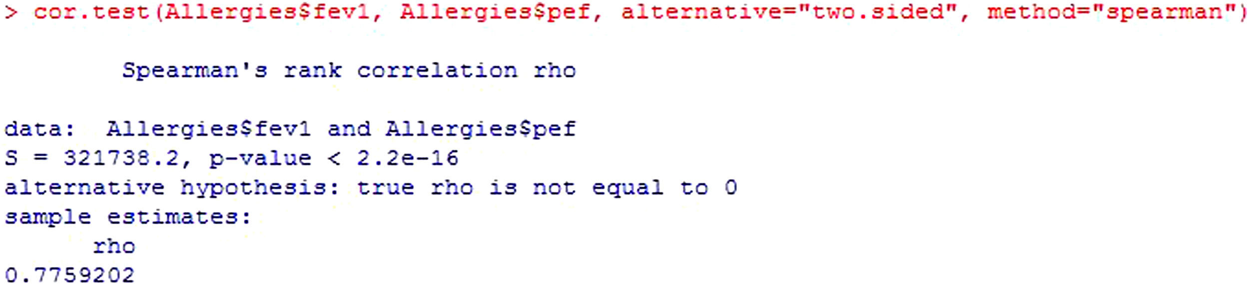
Following the initial description offered by the R Commander program, the value of the statistic is presented (S), along with the significance of the test (p-value) and the correlation coefficient (rho) (Figure 12).

The value of the statistic, S, is the correlation coefficient of the Spearman ranges and takes values of −1 to 1 – zero meaning no correlation.
The correlation coefficient (rho) is an index with possible values of 0 to 1, or of 0 to 100 when converted to percentages. The closer the value to 1 or 100, the greater the correlation between the variables, i.e., the closer the association between them.
The square of this coefficient is the percentage variability of fev explained by pef, i.e., the percentage to which the variable pef explains the dependent variable fev. The larger the value, the more one variable explains the other.
In bivariate correlations, as in the present case, the correlation coefficient must be greater than 50% in order to accept good correlation.11
The sign of rho indicates that the relationship is direct, i.e., increases in fev imply increases in pef. In contrast, if the coefficient were negative, the relationship would be indirect, i.e., increases in fev imply reductions in pef. Since p<0.05, it would be concluded that the correlation between the study variables is statistically significant.
In some cases correlations of under 50% yield significant p-values, i.e., p<0.05. In such cases it is important to analyze the correlation graphically and determine whether such significance truly exists. If there is indeed a correlation between the variables, a linear relationship will be seen.
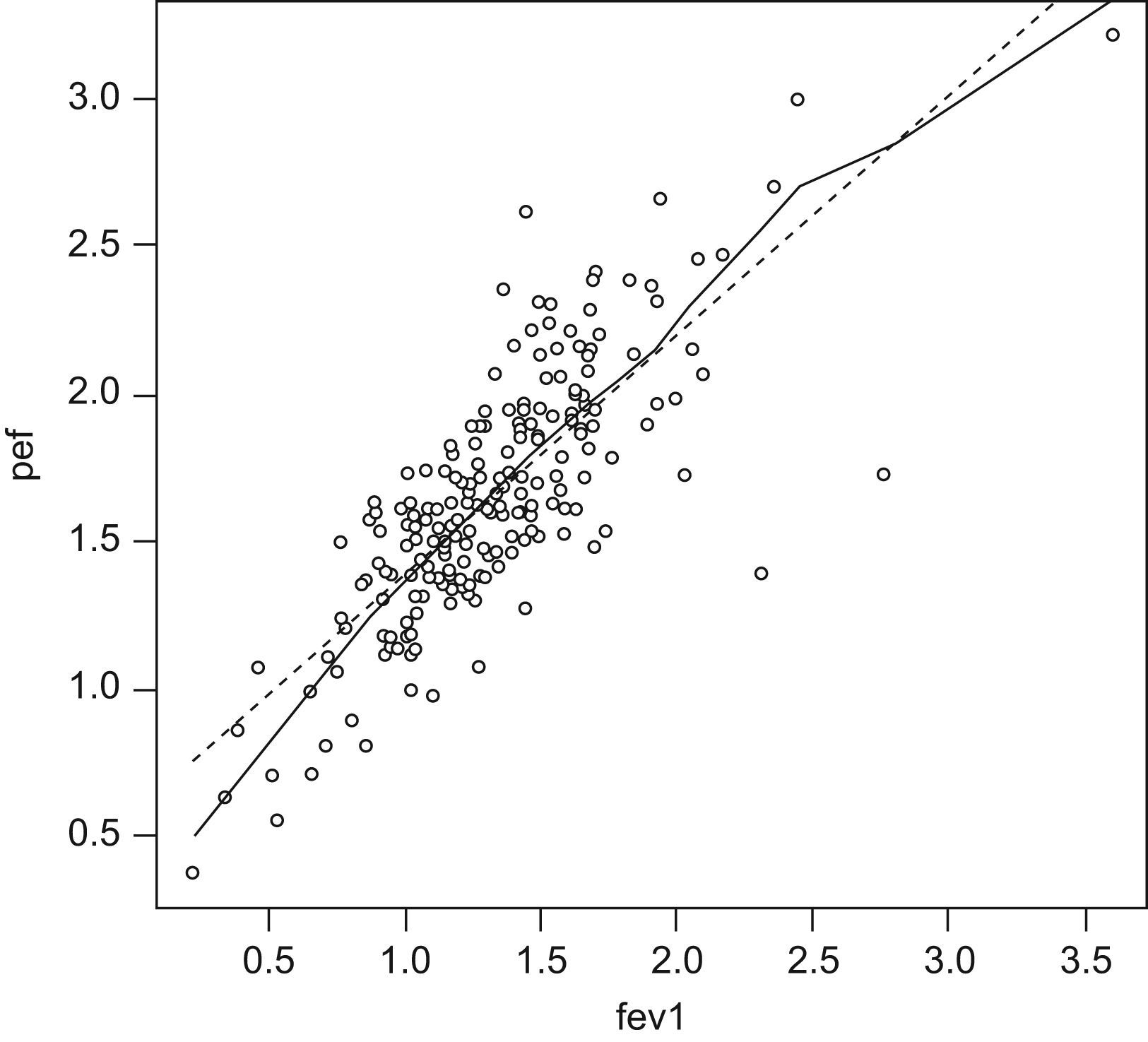
Figure 13 graphically shows the correlation between the study variables.

This figure shows that as the independent variable fev increases, the dependent variable pef increases in a linear manner. The plotted points are seen to “fit” the straight line (there would be no such fitting with rho values of under 50%).
The next step in the correlation analysis and in the above figure is to adjust the equation of the straight line. Linear regression will be explained in later articles.
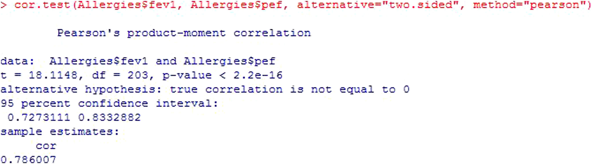
Continuing with the bivariate correlations and statistics according to whether they meet the applicability conditions or not, and based on the central limit theorem, if the sample in relation to each of the study variables is larger than 30, we can apply the Parametric Pearson test (Figure 14).

According to the mentioned theorem, we could apply a parametric test since n>30 for both variables (Figure 15). The starting interpretation is the same as that of the Spearman test – simply the notation is modified.

The Pearson statistic, t, takes values of −1 to 1 and measures the linear relationship between two quantitative variables. For samples of n>20, it constitutes an approximation of the Student's t-test.
Both the t statistic and its degrees of freedom (df) serve to calculate the p-value. The existing programs already offer the calculated value; consequently, they are simply used for informative purposes.
Since p<0.05, we assume that the correlation, cor, between the two variables (78.6%) is statistically significant. The square of this correlation indicates the variability of the dependent variable explained by the independent variable.
The sign in turn shows that the correlation between the two variables is direct or positive, i.e., when one increases so does the other.
In the output, the confidence interval of the correlation is also shown.6
It must be taken into account that neither the correlations nor their signs or the p-value present important changes according to the statistic used.
Testing two independent proportionsHaving addressed the hypothesis test involving numerical or quantitative variables, we focus now in testing hypothesis for qualitative data.
In response to the question of whether boys are more susceptible to allergy than girls, the corresponding contrast of hypothesis is as follows:
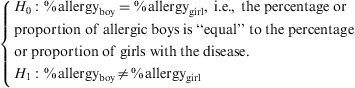
The statistic used to test difference between proportions and thus answer the question is the chi-squared statistic for tables of over 2×2 and the Yates correction for continuity for 2×2 tables. The latter is a correction of the chi-squared statistic when the variables to be related are both dichotomic.
The statistic value is obtained from the contingency tables, which are crossed tables in which the dependent variable (in our case having or not having allergy) is represented in the rows and the independent variable (sex) in the columns.
The requirements for using the chi-squared test are that the variables to be related are qualitative or categorical, and the independence of the sample, i.e., different variables measured at the same point in time.
In the same way as normality was the basic condition for when there were numerical variables in the hypothesis, the condition for qualitative variables is that there are sufficient observations in each of the cells of the contingency table.
How can we know if the number of observations is sufficient?
Calculation of the expected frequency of each cell provides the information.
The expected frequency for each cell is calculated from the multiplication of the marginal values of the table divided among the total, and in order for the statistic to be valid, no more than 20% of the cells can have an expected frequency of under 5.
What happens if more than 20% of the cells have expected frequencies of under 5?
- 1.
For tables of over 2×2, the chi-squared test is not valid, and the only solution would be to group categories of the variables or increase the sample.
- 2.
For 2×2 tables, the Yates continuity statistic can be corrected from the Fisher exact test.
Any statistical package offers the options of all these tests, and the use of one test or another will depend on whether one set of conditions or another are met.
Example: Continuing with the allergic patients database, a study is made to determine whether the percentage of allergic subjects differs according to the sex of the patient.
Hypothesis testApplicability conditions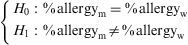
- •
The variables entered in the contrast are qualitative; one with two categories and the other with three, and the sample is independent.
- •
For tables of over 2×2 (in this case 2×3), the statistic to be used is the chi-squared test.
- •
No more than 20% of the cells of the 2×3 contingency table can have an expected frequency of under 5 in order for the statistic to be valid. If this condition is not met, the solution would be to group categories, which would give rise to a loss of information, or to increase the sample.
- •
Grouping of the categories must be done on the basis of clinical criteria.
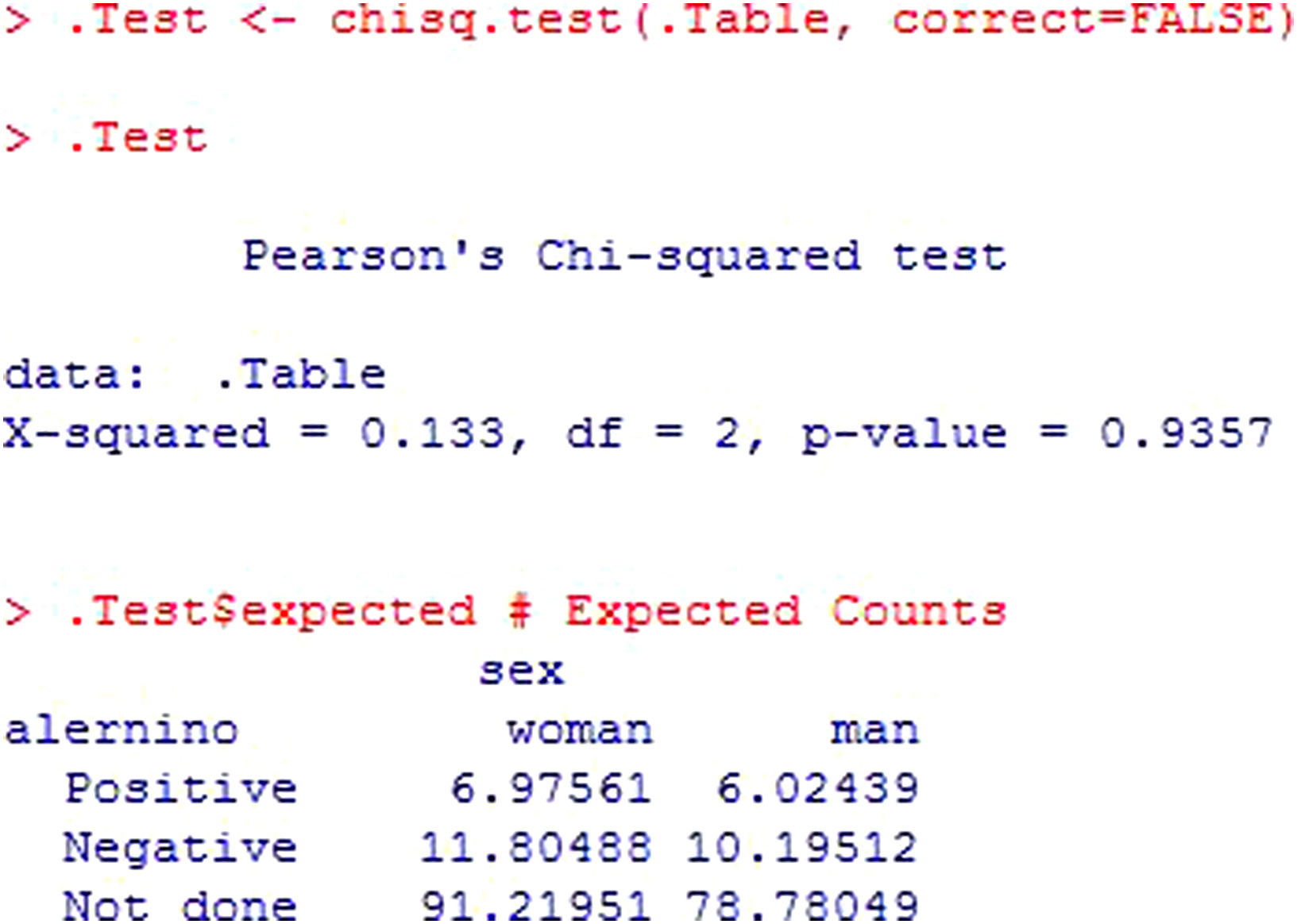
The output (Figure 16) indicates the calculated statistic (X-squared), the degrees of freedom (df) and the significance value of the statistic (p-value). Posteriorly, the table of expected frequencies is shown, allowing us to conclude whether the value of the statistic is valid or not.

In this case, 100% of the expected frequencies are over 5; as a result, it can be concluded that there are no statistically significant differences in the number of allergic subjects according to sex (p>0.05).
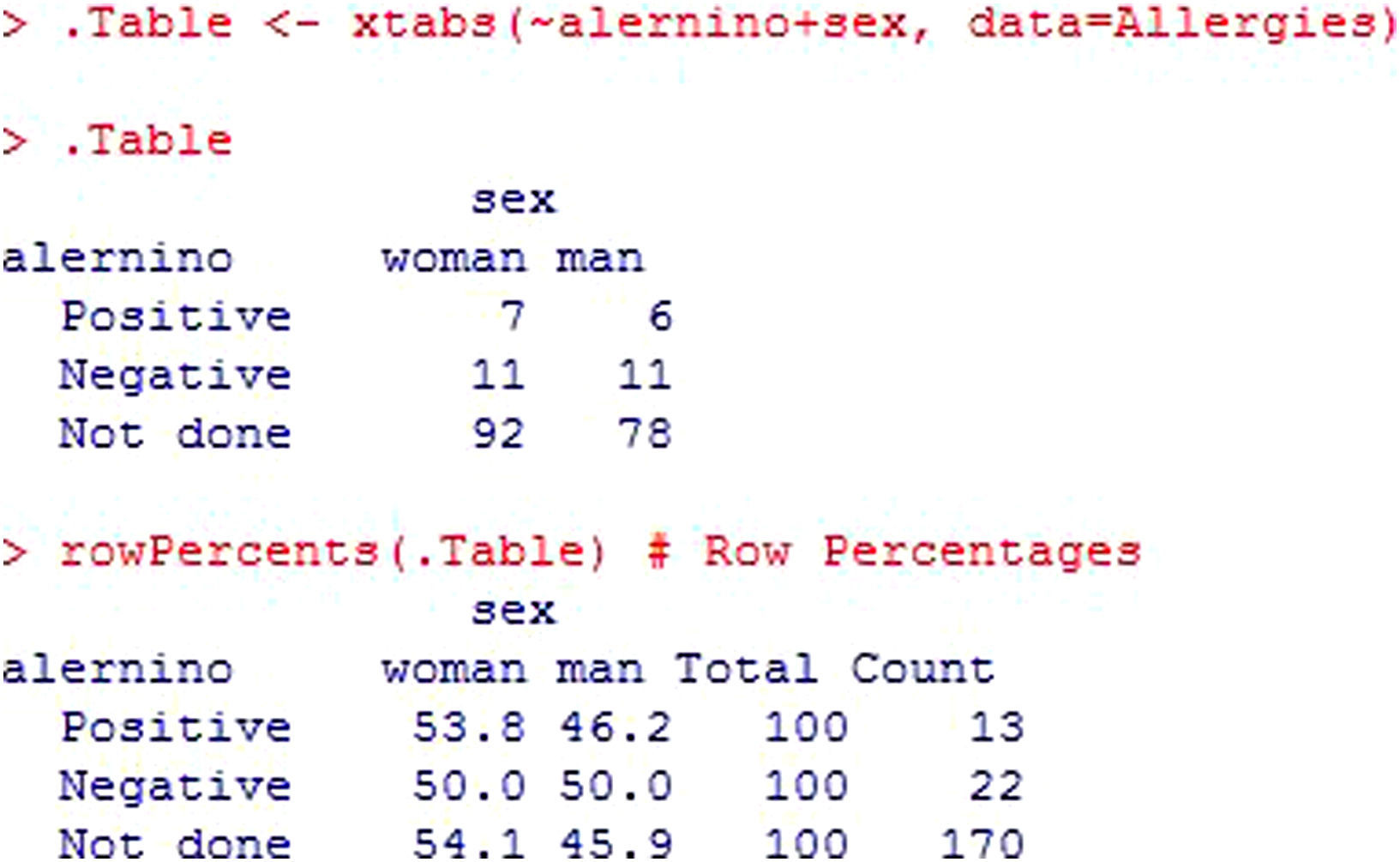
The rest of the analysis is shown in Figure 17. The first table corresponds to the contingency table in which the absolute frequencies of each cell are shown. We have 7 girls with a positive result in the allergy tests, versus 6 boys. Apart from the absolute frequencies, the relative frequencies are shown – in this case calculated by rows. The percentages can be calculated with respect to the absolute frequency of girls with a positive result, by rows (over 13), by columns (over 120), or the total (over 170).
Testing two dependent proportions.")
We now consider two qualitative variables in dependent samples, i.e., the same variables measured at different points in time.
The question is raised of whether a given intervention reduces the percentage of allergic subjects in the study population. Initially we measure the percentage of allergic individuals; the intervention is carried out; and posteriorly measurement is again performed to determine whether the patients are allergic or not. The same qualitative variable is involved (allergic or not allergic), at different timepoints (baseline and after the intervention).
The hypothesis test for this question would be as follows:
In this example we have a 2×2 table for dependent samples. Thus, the statistic to be used for answering the question of whether the intervention reduces the percentage of allergic patients is the McNemar test. The output and reading of this test is similar to that of the chi-squared test.
For rxn tables, where r=n, the contrast statistic indicated is the Cochran test. Here again, the interpretation is similar to that of the chi-squared test.
Limitations of hypothesis testFrom the healthcare perspective, we should avoid excessive dependency upon statistical significance tests, given the misconception that the results obtained will have greater scientific rigor when accompanied by a p-value.12 Independently of statistical significance, the results obtained in any hypothesis test must be weighed against their clinical relevance. The clinical judgment of the researcher must establish the relevance of the results offered by the statistical tests used, on the basis of the magnitude of the differences, morbidity-mortality, or the seriousness of the disease, among other aspects to be considered.
Among the weaknesses of hypothesis testing, mention must be made of the arbitrary selection of a single cut-off point, or the dichotomic decision of whether a given treatment is effective or whether a given form of exposure constitutes a risk – when the most appropriate approach might be to view the situation on a continuous basis.13
The manuscript preparation uniformity criteria established by the Vancouver group call to avoid exclusive dependence upon hypothesis verification statistical tests, which must be accompanied by the appropriate indicators of error and uncertainty of the measures, such as the confidence intervals.14
Statistical softwareAs regards the available statistical software, and although a broad range of packages can be used, the examples in this article have been worked with the R Commander, of which there are many guides to facilitate learning software.15 The menu options for accessing the test carried out, by order of appearance in the article, are indicated below:
- •
Statistics→Summaries→Shapiro-Wilks normality test
- •
Statistics→Variances→Levene test
- •
Statistics→Means-t-test for independent samples
- •
Statistics→Non-parametric tests→Kruskal-Wallis test
- •
Statistics→Means→t-test for related data
- •
Statistics→Non-parametric tests→Wilcoxon test for paired samples
- •
Statistics→Means→Single-factor ANOVA
- •
Statistics→Non-parametric tests→Kruskal-Wallis test
- •
Statistics→Means→Multiple-factors ANOVA
- •
Statistics→Non-parametric tests→Friedman rank sum test
- •
Statistics→Summaries→Correlation test
- •
Graphs→Scatterplot
Statistics→Contingency table→Dual input table
The authors, Manuela Exposito-Ruiz and Sabina Pérez-Vicente, have Research Supporting Technician contracts financed by the Instituto de Salud Carlos III.
